Black-Scholes-Merton Model
Overview
The Black-Scholes-Merton (BSM) model provides a simple formula for computing the price of an option.
- It is derived in a fashion similar to the binomial option pricing model.
- A riskless portfolio is obtained by buying \(\smash{\Delta}\) shares of the underlying asset and shorting a single option.
- \(\smash{\Delta}\) represents \(\smash{\frac{\partial C}{\partial S}}\), where \(\smash{S}\) is the price of the underlying and \(\smash{C}\) is the price of the option.
- Unlike the binomial model, the BSM model \(\smash{\Delta}\) is only valid for an infinitesimal length of time.
BSM Assumptions
The BSM model depends on the following assumptions.
- The price of the underlying asset follows geometric Brownian motion with parameters \(\smash{\mu}\) and \(\smash{\sigma}\).
- There is no restriction on short selling.
- There are no transaction costs or taxes.
- All assets are perfectly divisible.
- The underlying doesn’t pay dividends.
- There are no riskless arbitrage opportunities.
- Asset trading occurs continuously.
- The risk-free rate, \(\smash{r}\) is constant and the same for all maturities.
BSM and Ito’s Lemma
Suppose the price of an asset follows geometric Brownian motion:
According to Ito’s lemma, the price of a derivative, \(\smash{f}\), follows:
A Riskless Portfolio
Consider a portfolio that is short one unit of the derivative and long \(\smash{\frac{\partial f}{\partial S}}\) units of the underlying:
Note that the portfolio is not affected by \(\smash{Z}\), so it is riskless.
A Riskless Portfolio
- The portfolio must earn the risk-free rate of return over period \(\smash{dt}\).
- This is the BSM differential equation.
Boundary Conditions
The BSM differential equation is true for any derivative that depends on \(\smash{S}\).
- Boundary conditions determine the price of a particular derivative.
- For example, the boundary condition for a call option is its terminal value: \(\smash{f = \max(S-X,0)}\).
- Likewise, the boundary condition for a put option is its terminal value: \(\smash{f = \max(X-S,0)}\).
BSM Price of Forward
Suppose that some time ago a forward contract was entered into with delivery price \(\smash{K}\) and maturity \(\smash{T}\).
- Recall that at intermediate date \(\smash{t}\) the value of the forward is \(\smash{f = S - K e^{-r(T-t)}}\).
- It follows:
- Substituting these into the BSM equation, \(\smash{rf = rS - rK e^{-r(T-t)}}\), which is true.
Risk-Neutral Valuation
A basic principle of asset pricing is that investors demand higher expected return, \(\smash{\mu}\), in the presence of higher volatility, \(\smash{\sigma}\).
- Note that \(\smash{\mu}\) doesn’t appear in the BSM differential equation.
- This means we can treat investors as if they are risk neutral.
- That is, we can value assets under the assumption that investors only demand expected return \(\smash{r}\), even though they aren’t really risk neutral.
- The practical implication is that once we compute future asset payoffs, we can discount them at the risk-free rate (implicitly assuming this is the rate of return that investors demand).
BSM Option Pricing Formulas
The BSM option pricing formulas are:
- These satisfy the BSM differential equation.
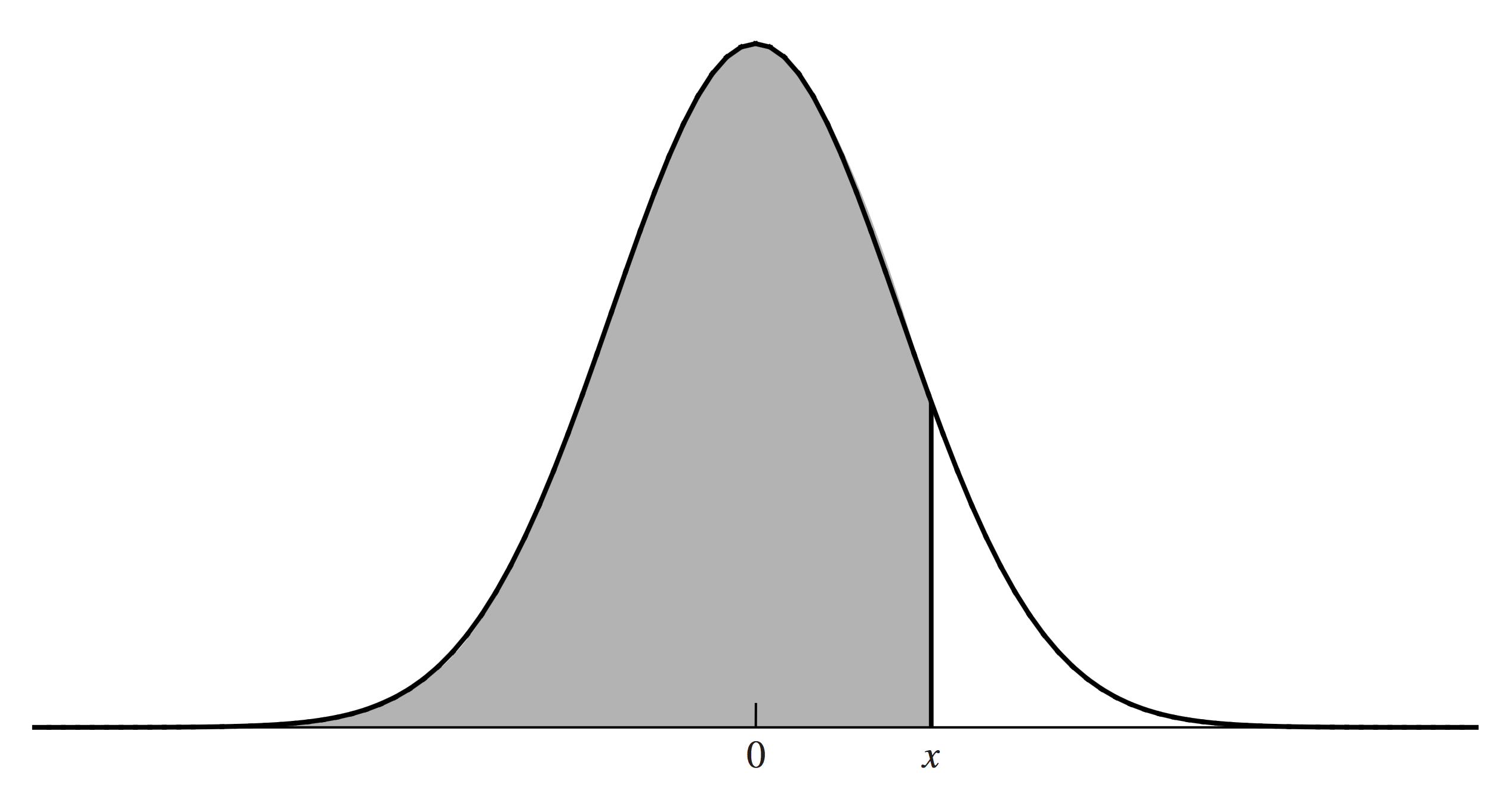
- \(\smash{\Phi(x)}\) represents the standard Normal CDF: \(\smash{P(X \leq x)}\) when \(\smash{X \sim N(0,1)}\).
- \(\smash{C}\) and \(\smash{P}\) are the prices of European call and put options on the underlying, \(\smash{S}\).
Normal CDF
Interpretation
Interpretation
The last equation above follows because, under risk-neutrality \(\smash{E\left[\log(S_T)\right] = \log(S_0) + (r - \sigma^2/2)T}\) and \(\smash{Sd\left(\log(S_T)\right) = \sigma \sqrt{T}}\):
Interpretation
\(\smash{\Phi(d_1)}\) is similar to \(\smash{\Phi(d_2)}\), but slightly harder to interpret.
- \(\smash{S_0\Phi(d_1) e^{rT}}\) is the expected asset price (under risk neutrality), conditional on the asset expiring with \(\smash{S_T \geq X}\).
- The expected payoff of the call option is:
- The present value of the call option expected payoff is:
Extreme Cases
Suppose the current stock price \(\smash{S_0}\) is very large relative to the strike \(\smash{X}\).
- In this case \(\smash{d_1}\) and \(\smash{d_2}\) are very large.
- As a result \(\smash{\Phi(d_1)}\) and \(\smash{\Phi(d_2)}\) approach 1.
- This causes the call option value to be \(\smash{S_0 - X
e^{-rT}}\).
- This is identical to a forward contract, which makes sense for a deep-in-the-money call.
- Likewise \(\smash{\Phi(-d_1)}\) and \(\smash{\Phi(-d_2)}\) approach 0.
- This causes the put option value to be 0.
Extreme Cases
Suppose \(\smash{\sigma \to 0}\).
- If \(\smash{S_0 > X e^{-rT}}\), then \(\smash{d_1 \to \infty}\) and \(\smash{d_2 \to \infty}\), causing \(\smash{\Phi(d_1) \to 1}\) and \(\smash{\Phi(d_2) \to 1}\).
- The result is a value of \(\smash{S_0 - X e^{-rT} > 0}\), which is identical to the riskless payoff \(\smash{\max(S_0 e^{rT} - X,0)}\).
- Likewise, if \(\smash{S_0 < X e^{-rT}}\), then \(\smash{d_1 \to -\infty}\) and \(\smash{d_2 \to -\infty}\), causing \(\smash{\Phi(d_1) \to 0}\) and \(\smash{\Phi(d_2) \to 0}\).
- The result is a value of \(\smash{0}\), which is identical to the riskless payoff \(\smash{\max(S_0 e^{rT} - X,0)}\).
Implied Volatility
Volatility, \(\smash{\sigma}\), is the single parameter of the BSM model that is not directly observed.
- Typically, the BSM equation is not used to compute an option price, but to compute an implied volatility, given an option price.
- For example, if \(\smash{C = 1.875}\), \(\smash{S_0 = 21}\), \(\smash{X = 20}\), \(\smash{r = 0.1}\) and \(\smash{T = 0.25}\), what is the value that \(\smash{\sigma}\) must take for the BSM equation to hold for a European call option?
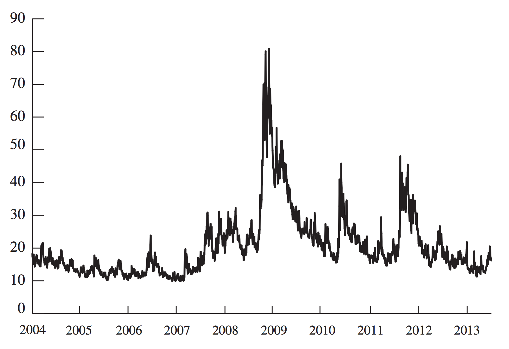
VIX Index
The VIX index is an index of implied volatilities for 30-day S&P 500 options (calls and puts).
- It is interpreted as the (annualized) one standard deviation move (in percentage) of the S&P 500 index over the next 30 days.
- Options and futures trade on the VIX itself (as well as the S&P 500).
Historical VIX