Wiener Processes¶

Stochastic Processes¶

A stochastic process is a collection of random variables, indexed by time.

More simply, it can be thought of as a single random variable that evolves dynamically with time.

Stochastic processes can be discrete/continuous time: either they evolve discretely or continuously.

They can be discrete/continuous value: at each time, they are drawn from either a discrete or continuous probability distribution.

We will develop a continuous time/continuous value model for asset prices.
- Note that we only observe discrete value and discrete time observations for actual asset prices.

Properties of Expected Value¶

Given random variables $\smash{X}$ and $\smash{Y}$, define a new random variable $\smash{Z = X + Y}$. Then:

\[\begin{split}\begin{align} E[Z] & = E\left[X + Y \right] = E[X] + E[Y]. \end{align}\end{split}\]

Suppose $\smash{E[X] = E[Y] = \mu}$. Then:

\[\begin{split}\begin{align} E[Z] & = E[X] + E[Y] = 2 \mu. \end{align}\end{split}\]

Properties of Expected Value¶

Extending the prior result, given random variables $\smash{\left\{X_i\right\}_{i=1}^n}$, define a new random variable $\smash{Z = \sum_{i=1}^n X_i}$. Then:

\[\begin{split}\begin{align} E[Z] & = E\left[\sum_{i=1}^n X_i \right] = \sum_{i=1}^n E[X_i]. \end{align}\end{split}\]

Suppose $\smash{E[X_i] = \mu, \,\, i=1,\ldots,n}$. Then:

\[\begin{split}\begin{align} E[Z] & = \sum_{i=1}^n E[X_i] = \sum_{i=1}^n \mu = n \mu. \end{align}\end{split}\]

Properties of Variance¶

Given random variables $\smash{X}$ and $\smash{Y}$, define a new random variable $\smash{Z = X + Y}$. Then:

\[\begin{split}\begin{align} Var(Z) & = Var\left(X + Y \right) = Var(X) + Var(Y) + 2 Cov(X,Y). \end{align}\end{split}\]

Suppose $\smash{Var(X) = Var(Y) = \sigma^2}$ and that they are independent $\smash{(Cov(X,Y)=0)}$. Then:

\[\begin{split}\begin{align} Var(Z) & = Var(X) + Var(Y) = 2 \sigma^2 \\ \Rightarrow Sd(Z) & = \sqrt{Var(Z)} = \sqrt{2} \sigma. \end{align}\end{split}\]

Properties of Variance¶

Extending the prior result, given random variables $\smash{\left\{X_i\right\}_{i=1}^n}$, define a new random variable $\smash{Z = \sum_{i=1}^n X_i}$. Then:

\[\begin{split}\begin{align} Var(Z) & = Var\left(\sum_{i=1}^n X_i \right) = \sum_{i=1}^n Var(X_i) + 2 \sum_{i=1}^{n-1} \sum_{j=i+1}^n Cov(X_i,X_j). \end{align}\end{split}\]

Suppose $\smash{Var(X_i) = \sigma^2, \,\, i=1,\ldots,n}$ and that each random variable is independent of the others $\smash{(Cov(X_i,X_j)=0, \,\, i \neq j)}$. Then:

\[\begin{split}\begin{align} Var(Z) & = \sum_{i=1}^n Var(X_i) = \sum_{i=1}^n \sigma^2 = n \sigma^2 \\ \Rightarrow Sd(Z) & = \sqrt{Var(Z)} = \sqrt{n} \sigma. \end{align}\end{split}\]

Normal Random Variables¶

Suppose $\smash{X_i \sim N(\mu,\sigma), \,\, i=1,\ldots, n}$.

Define a new random variable $\smash{Z = \sum_{i=1}^n X_i}$.

We already know $\smash{E[Z] = n\mu}$ and $\smash{Sd(Z) = \sqrt{n} \sigma}$.

However, the sum of Normals is also Normal: $\smash{Z \sim N\left(n\mu, \sqrt{n} \sigma\right)}$.

Additive Normal Example¶

Suppose the monthly return on an asset is Normally distributed for each month over the next year.

We will assume the expected value is 1% and standard deviation is 5% and that returns across months are independent:

\[\begin{align} R_i \stackrel{i.i.d.}{\sim} N(0.01,0.05), \,\,\,\, i = 1,\ldots, 12. \end{align}\]

The annual return is the sum of monthly returns: $\smash{R_a = \sum_{i=1}^{12} R_i}$.

The distribution of the annual return is $\smash{R_a \sim N(0.12,0.1732)}$.

Additive Normal Example¶

Note that we can also work backwards.

Suppose you know that the annual expected return is $\smash{\mu_a = 0.12}$, the annual standard deviation is $\smash{\sigma_a = 0.1732}$ and that monthly returns are independent.

The monthly expected return and standard deviation are:

\[\begin{split}\begin{align} \mu_m & = \frac{\mu_a}{n} = \frac{0.12}{12} = 0.01 \\ \sigma_m & = \frac{\sigma_a}{\sqrt{n}} = \frac{0.1732}{\sqrt{12}} = 0.05. \end{align}\end{split}\]

Wiener Process¶

A random variable $\smash{Z(t)}$ follows a Wiener process if:

During a short time interval $\smash{\Delta t}$,

\[\begin{split}\begin{align} \Delta Z(t) & = Z(t) - Z(t-\Delta t) = \varepsilon \sqrt{\Delta t}, \,\,\, \varepsilon \sim N(0,1). \end{align}\end{split}\]

The values of $\smash{\Delta Z(t)}$ for any two short intervals $\smash{\Delta t}$ are independent.

As $\smash{\Delta t \to 0}$, we use the notation $\smash{dZ = \varepsilon \sqrt{dt}}$.

Moments of the Wiener Process¶

What are the first two moments of $\smash{\Delta Z(t)}$?

\[\begin{split}\begin{align} E\left[\Delta Z(t)\right] & = E\left[\varepsilon \sqrt{\Delta t}\right] = \sqrt{\Delta t} E\left[\varepsilon\right] = 0 \\ Var\left(\Delta Z(t)\right) & = Var\left(\varepsilon \sqrt{\Delta t}\right) = \Delta t Var\left(\varepsilon\right) = \Delta t \\ Sd\left(\Delta Z(t)\right) & = Sd\left(\varepsilon \sqrt{\Delta t} \right) = \sqrt{\Delta t} Sd\left(\varepsilon\right) = \sqrt{\Delta t}. \end{align}\end{split}\]

Wiener Process Over Long Horizon¶

Consider the evolution of $\smash{Z(t)}$ over a longer horizon $\smash{T}$.

Divide the time interval $\smash{(0,T)}$ into $\smash{N}$ small intervals of equal length $\smash{\Delta t}$.

Then:

\[\begin{split}\begin{align} Z(T) - Z(0) & = \sum_{i=1}^N \varepsilon_i \sqrt{\Delta t}, \,\,\, \varepsilon_i \stackrel{i.i.d.}{\sim} N(0,1). \end{align}\end{split}\]

Wiener Process Over Long Horizon¶

The resulting moments are:

\[\begin{split}\begin{align} E\left[Z(T) - Z(0)\right] & = \sum_{i=1}^N \sqrt{\Delta t} E[\varepsilon_i] = 0 \\ Var\left(Z(T) - Z(0)\right) & = \sum_{i=1}^N \Delta t Var(\varepsilon_i) = T \\ Sd\left(Z(T) - Z(0)\right) & = \sum_{i=1}^N \sqrt{\Delta t} Sd(\varepsilon_i) = \sqrt{T}. \end{align}\end{split}\]

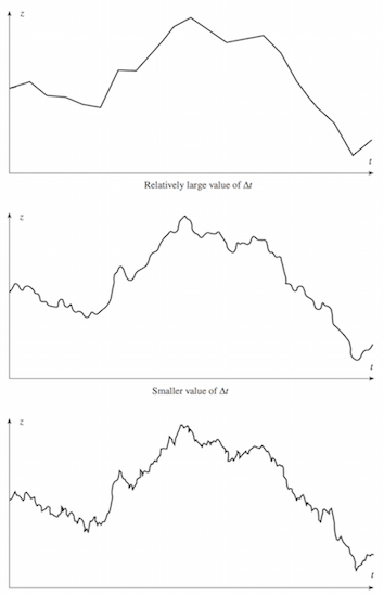
Wiener Process Sample Paths¶

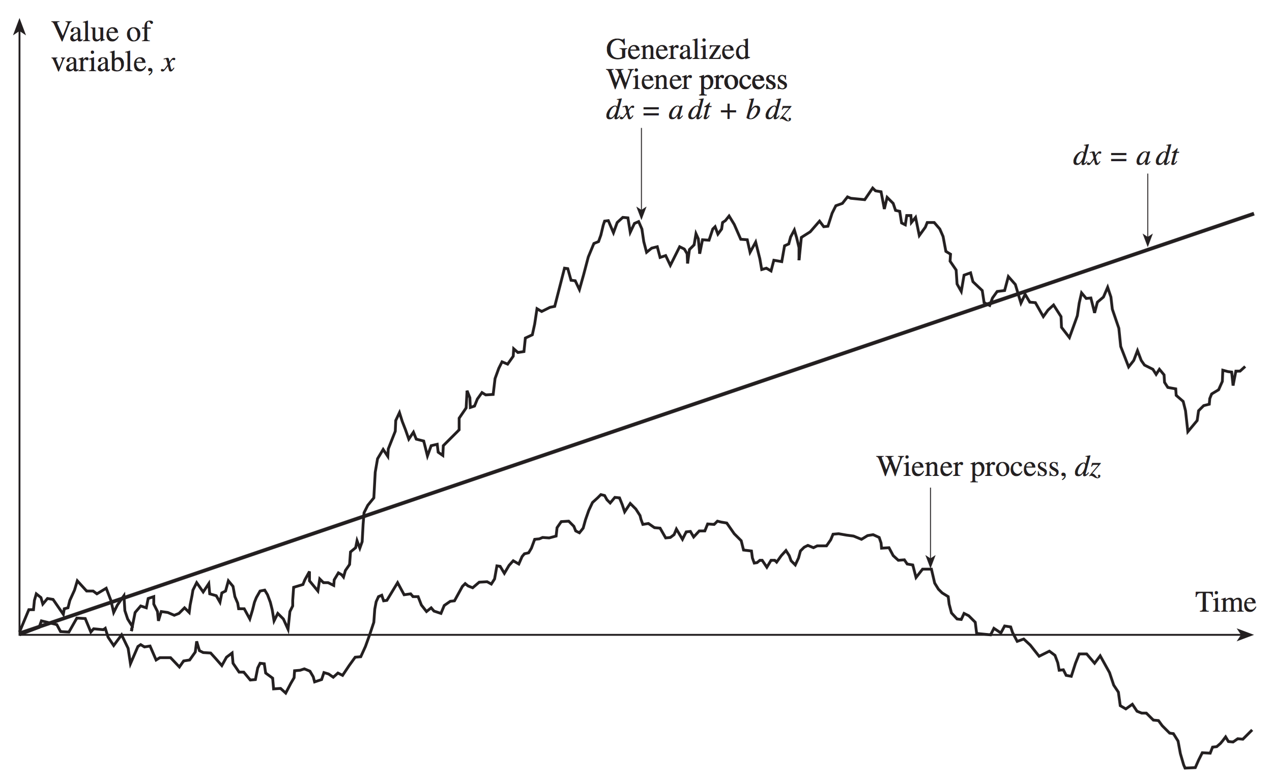
Generalized Wiener Process¶

Consider the generalized Wiener process:

\[\begin{split}\begin{align} dX & = a dt + b dZ. \end{align}\end{split}\]

$\smash{a}$ is the drift rate and $\smash{b^2}$ is the variance rate.

The basic Wiener process has drift rate zero and unit variance rate.

Generalized Wiener Process¶

In discrete time, the generalize Wiener process is

\[\begin{split}\begin{align} \Delta X & = a \Delta t + b \varepsilon \sqrt{\Delta t}. \end{align}\end{split}\]

The moments are:

\[\begin{split}\begin{align} E[\Delta X] & = a \Delta t \\ Var(\Delta X) & = b^2 \Delta t \\ Sd(\Delta X) & = b \sqrt{\Delta t}. \end{align}\end{split}\]

Wiener Process Comparison¶

Ito Process¶

An Ito process is a generalization of a generalized Wiener process:

\[\begin{split}\begin{align} dX & = a(X,t) dt + b(X,t) dZ. \end{align}\end{split}\]

The drift rate and variance rate are functions of the process value and time - i.e. they are variable.

In discrete time:

\[\begin{split}\begin{align} \Delta X & = a(X,t) \Delta t + b(X,t) \varepsilon \sqrt{\Delta t}. \end{align}\end{split}\]

The discrete time analog requires an approximation: the drift and variance rate are constant over small intervals $\smash{\Delta t}$.

Model for Asset Prices¶

We will use an Ito process as a model for asset prices.

We think of percentage returns as being constant for a particular asset.

This means that the size of the moves (the drift) changes with the level of the price.

Variance also typically changes with the level of asset prices.

This means an Ito process is a better model than a generalized Wiener process.

Model for Asset Prices¶

We will employ the following Ito process:

\[\begin{split}\begin{align} dS & = \mu S dt + \sigma S dZ. \end{align}\end{split}\]

The drift rate function takes the specific form: $\smash{a(S,t) = \mu S}$.
- The drift rate increases proportionally with the asset price and does not depend on time.

The variance rate function takes the specific form: $\smash{b^2(S,t) = \sigma^2 S^2}$.
- The volatility, $\smash{b(S,t) = \sigma S}$, increases proportionally with the asset price and does not depend on time.

This form of an Ito process is known as geometric Brownian motion.

Geometric Brownian Motion¶

Geometric Brownian motion can also be written as:

\[\begin{split}\begin{align} \frac{dS}{S} & = \mu dt + \sigma dZ. \end{align}\end{split}\]

$\smash{\frac{dS}{S}}$ is effectively the return.

Note that returns evolve as a generalized Wiener process (constant drift and variance rates).

$\smash{\mu}$ and $\smash{\sigma}$ are the expected return and volatility of the asset.

Geometric Brownian Motion¶

In discrete time, geometric Brownian motion is described as:

\[\begin{split}\begin{align} \frac{\Delta S}{S} & = \mu \Delta t + \sigma \varepsilon \sqrt{\Delta t}. \end{align}\end{split}\]

This means $\smash{\frac{\Delta S}{S} \sim N(\mu \Delta t, \sigma \sqrt{\Delta t})}$.

Parameter Estimation¶

We can estimate the parameters $\smash{\mu}$ and $\smash{\sigma}$ from historical data.

Set an interval of time, $\smash{\Delta t}$ in years (days, weeks, months, etc).

Collect $\smash{n+1}$ price observations for the beginning and end of each interval.

Compute $\smash{n}$ returns for the invervals.

Set $\smash{\hat{\mu}}$ and $\smash{\hat{\sigma}}$ to the sample mean and sample standard deviation of the returns.

$\smash{\hat{\mu}}$ is an estimate of $\smash{\mu \Delta t}$, not $\smash{\mu}$.

$\smash{\hat{\sigma}}$ is an estimate of $\smash{\sigma \sqrt{\Delta t}}$, not $\smash{\sigma}$.

Simulating Geometric Brownian Motion¶

Let’s estimate the daily mean and standard deviation of Lockheed Martin (LMT) returns using data prior to January 1, 2015:

> library(quantmod)
> getSymbols("LMT",src="yahoo", from="2010-01-01", to="2014-12-31")
> lmtRets = dailyReturn(LMT)
> mu = mean(lmtRets)
> sigma = sd(lmtRets)
> cat(mu,sigma)
0.0008037858 0.01122918

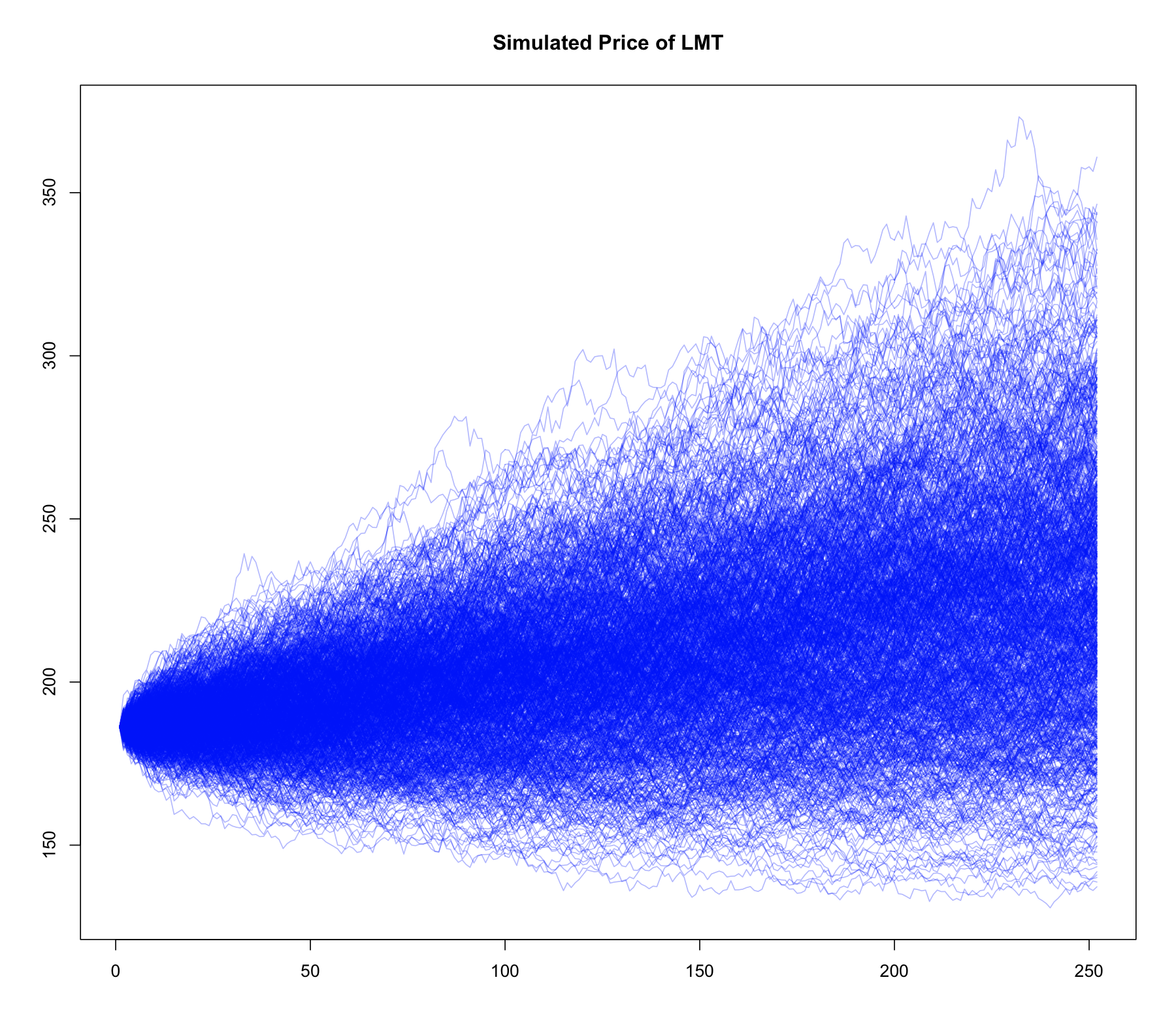
We now simulate 1000 price paths of one year (250 trading days) starting on Jan 2, 2015:

> nSim = 1000
> nDays = 252
> S0 = 186.21 # price on Jan 2, 2015
> S = matrix(0,nrow=nDays,ncol=nSim)
> for(ix in 1:nSim){
+    SVec = rep(0,nDays)
+    SVec[1] = S0
+    for(jx in 2:nDays){
+            DeltaS = mu*SVec[jx-1] + sigma*SVec[jx-1]*rnorm(1)
+            SVec[jx] = SVec[jx-1]+DeltaS
+    }
+     S[,ix] = SVec
+ }
> matplot(S,type='l',col=rgb(0,0,1,0.3),lty=1,ylab='',main='Simulated Price of LMT')

Simulating Geometric Brownian Motion¶

The closing price on Jan 4, 2016 was $\smash{\$211.61}$.

Ito’s Lemma¶

Suppose $\smash{X}$ follows and Ito process:

\[\begin{split}\begin{align} dX & = a(X,t) dt + b(X,t) dZ. \end{align}\end{split}\]

For some function $\smash{G(X,t)}$, Ito’s lemma says:

\[\begin{split}\begin{align} dG & = \left(\frac{\partial G}{\partial X} a(X,t) + \frac{\partial G}{\partial t} + \frac{1}{2} \frac{\partial^2 G}{\partial X^2} b(X,t)^2 \right) dt + \frac{\partial G}{\partial X} b(X,t) dZ. \end{align}\end{split}\]

Ito’s Lemma¶

Ito’s lemma says that $\smash{G(X,t)}$ is an Ito process with drift and variance rates

\[\begin{split}\begin{gather} \frac{\partial G}{\partial X} a(X,t) + \frac{\partial G}{\partial t} + \frac{\partial^2 G}{\partial X^2} b(X,t) \\ \left(\frac{\partial G}{\partial X}\right)^2 b(X,t)^2. \end{gather}\end{split}\]

Ito’s Lemma for Geometric Brownian Motion¶

Recall our model for stock prices:

\[\begin{split}\begin{align} dS & = \mu S dt + \sigma S dZ. \end{align}\end{split}\]

In this case, Ito’s lemma says that $\smash{G(S,t)}$ follows:

\[\begin{split}\begin{align} dG & = \left(\frac{\partial G}{\partial S} \mu S + \frac{\partial G}{\partial t} + \frac{1}{2} \frac{\partial^2 G}{\partial S^2} \sigma^2 S^2 \right) dt + \frac{\partial G}{\partial S} \sigma S dZ. \end{align}\end{split}\]

Application to Forward Contracts¶

Recall the formula for the value of a forward contract (given current time $\smash{t}$ and horizon $\smash{T-t}$):

\[\begin{align} F = S e^{r(T-t)}. \end{align}\]

In this case $\smash{F = G(S,t)}$.

The derivatives are

\[\begin{split}\begin{align} \frac{\partial F}{\partial S} & = e^{r(T-t)}, \,\,\,\, \frac{\partial^2 F}{\partial S^2} = 0, \,\,\,\, \frac{\partial F}{\partial t} = -r Se^{r(T-t)}. \end{align}\end{split}\]

Application to Forward Contracts¶

Following Ito’s lemma,

\[\begin{split}\begin{align} dF & = \left(e^{r(T-t)} \mu S - r S e^{r(T-t)} \right) dt + e^{r(T-t)} \sigma S dZ \\ & = (\mu - r) F dt + \sigma F dZ. \end{align}\end{split}\]

Distribution of Prices¶

What is the distribution of $\smash{S}$ if it follows geometric Brownian motion?

We know that returns, $\smash{\frac{dS}{S}}$, are Normal.

Let’s use Ito’s lemma to derive the law of motion of $\smash{G(S,t) = \ln(S)}$:

\[\begin{split}\begin{align} \frac{\partial G}{\partial S} & = \frac{1}{S} \,\,\,\, \frac{\partial^2 G}{\partial S^2} = -\frac{1}{S} \,\,\,\, \frac{\partial G}{\partial t} = 0 \\ \Rightarrow dG & = \left(\mu - \frac{\sigma^2}{2} \right) dt + \sigma dZ. \end{align}\end{split}\]

$\smash{\ln(S)}$ follows a generalized Wiener process with drift rate $\smash{\mu - \frac{\sigma^2}{2}}$ and variance rate $\smash{\sigma^2}$.

Distribution of Prices¶

The discrete analog to the process for $\smash{\Delta \ln(S)}$ is

\[\begin{split}\begin{align} \Delta \ln(S) & = \left(\mu - \frac{\sigma^2}{2} \right) \Delta t + \sigma \varepsilon \sqrt{\Delta t}. \end{align}\end{split}\]

For $\smash{\Delta t = T}$, $\smash{\Delta \ln(S) = \ln(S_T) - \ln(S_0)}$, which results in:

\[\begin{split}\begin{align} \ln(S_T) - \ln(S_0) \sim N\left(\left(\mu - \frac{\sigma^2}{2}\right)T, \sigma \sqrt{T}\right) \\ \Rightarrow \ln(S_T) \sim N\left(\ln(S_0) + \left(\mu - \frac{\sigma^2}{2}\right)T, \sigma \sqrt{T}\right) \\ \end{align}\end{split}\]

This means that prices are lognormally distributed.

Lognormal Distribution¶

Suppose $\smash{S_T \sim LN\left(\ln(S_0) + \left(\mu - \frac{\sigma^2}{2}\right)T, \sigma \sqrt{T}\right)}$.

By defintion, this means $\smash{\ln(S_T) \sim N\left(\ln(S_0) + \left(\mu - \frac{\sigma^2}{2}\right)T, \sigma \sqrt{T}\right)}$.

It can be shown that the mean and variance of $\smash{S_T}$ are

\[\begin{split}\begin{align} E[S_T] & = S_0 e^{\mu T} \\ Var(S_T) & = S_0^2 e^{2\mu T} \left(e^{\sigma^2 T}-1\right). \end{align}\end{split}\]

Simulation Distribution¶

We can check that our simulated geometric Brownian motion results in a lognormal distribution for LMT prices.

> lnMean = S0*exp(mu*nDays)
> lnSD = S0*exp(mu*nDays)*sqrt(exp((sigma^2)*nDays)-1)
> cat(lnMean,mean(S[nDays,]))
228.019 230.529
> cat(lnSD,sd(S[nDays,]))
40.97119 43.21174

Simulation Distribution¶

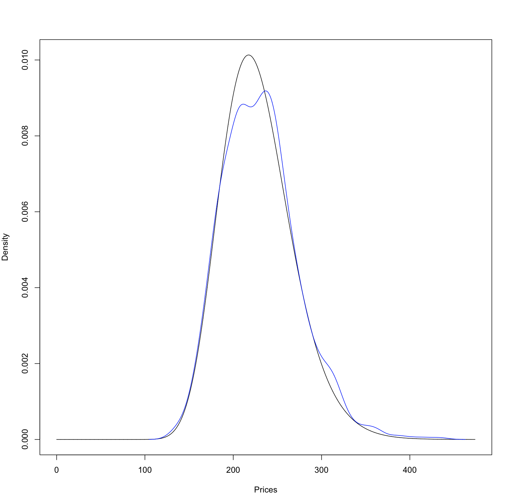
We can also plot the theoretical lognormal and the empirical distribution of LMT prices.

> meanOfLog = log(S0) + (mu-(sigma^2)/2)*nDays
> sdOfLog = sigma*sqrt(nDays)
> priceGrid = seq(0,lnMean+6*lnSD,length=10000)
> theoreticalDens = dlnorm(priceGrid,meanOfLog,sdOfLog)
> empiricalDens = density(S[nDays,])
> plot(priceGrid,theoreticalDens,type='l',xlab='Prices',ylab='Density')
> lines(empricalDens,col='blue')