Binomial Trees¶

Random Walk¶

A random walk is a stochastic process the evolves in the following manner:

\[\begin{split}\begin{align} Y_t & = Y_{t-1} + \varepsilon_t. \end{align}\end{split}\]

If $\smash{\varepsilon_t \sim N(0,1)}$, then $\smash{Y_t}$ is a continuous random variable and is a referred to as a Gaussian random walk.

If $\smash{\varepsilon_t}$ is drawn from a discrete distribution, then $\smash{Y_t}$ is also a discrete random variable.

We will refer to $\smash{\varepsilon_t}$ as the innovation or shock.

Binomial Distribution¶

Suppose a random variable $\smash{X}$ can only take one of two values $\smash{X_u}$ and $\smash{X_d}$.

If $\smash{P(X = X_u) = p}$ and $\smash{P(X = X_d) = 1-p}$, then $\smash{X}$ follows a Bernoulli distribution with parameter $\smash{p}$.

In notation: $\smash{X \sim Bernoulli(p)}$.

The sum of $\smash{n}$ independent Bernoulli random variables is a Binomial random variable with parameters $\smash{n}$ and $\smash{p}$.

In notation: if $\smash{Y_t = \sum_{i=t-n}^t X_i}$ then $\smash{Y_t \sim Binomial(n,p)}$.

Bernoulli Random Walk¶

A very simple model of stock prices assumes that they follow a random walk with Bernoulli innovations:

\[\begin{split}\begin{align} P_t & = P_{t-1} + \varepsilon_t, \,\,\,\, \varepsilon_t \sim Bernoulli(p). \end{align}\end{split}\]

Interpretation: The stock price can only move to one of two values at each time period.

This model is useful for valuing options on the asset.

Binomial Tree Example¶

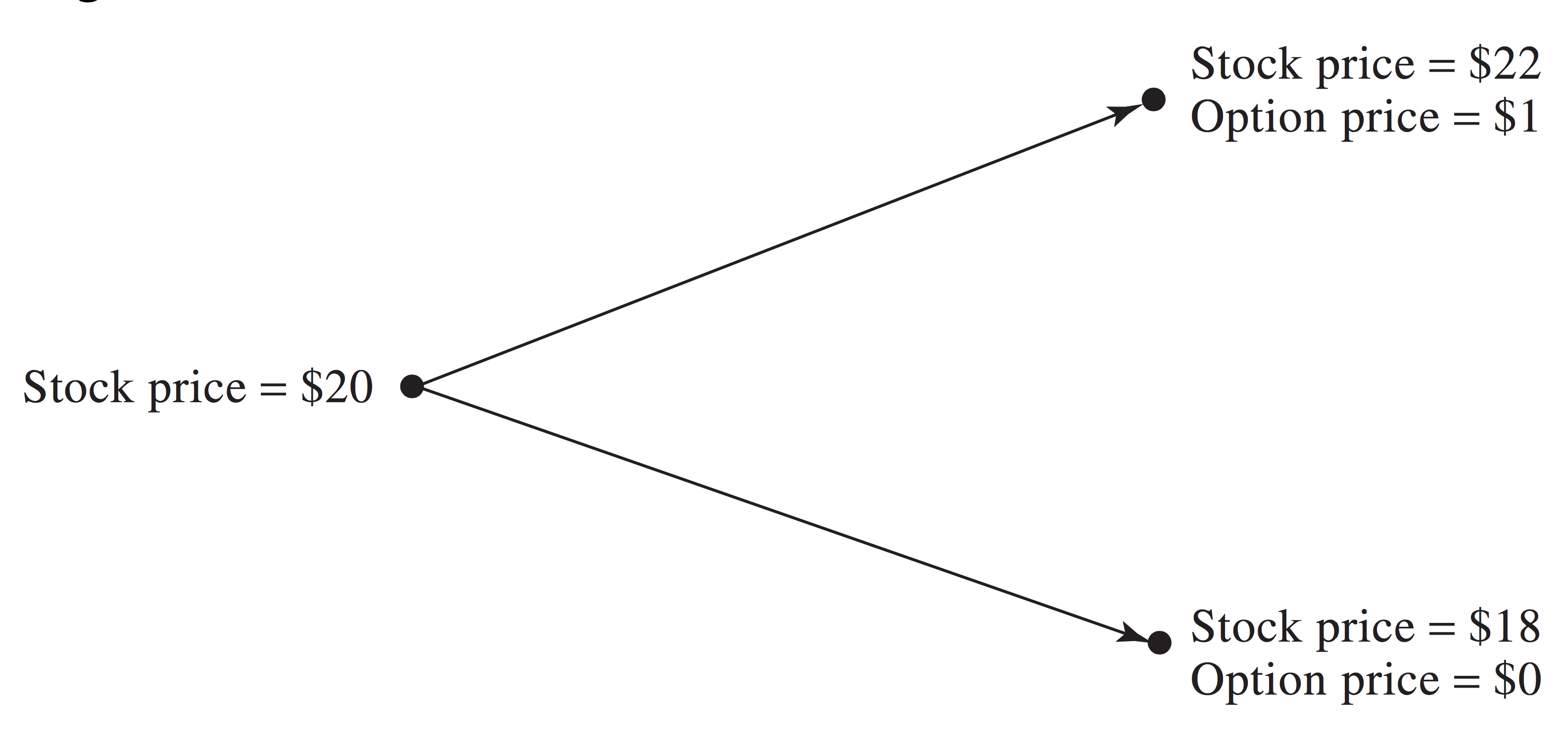
Suppose a stock price is currently $\smash{\$20}$ and that in three months it will either be $\smash{\$18}$ or $\smash{\$22}$.

You would like to buy a call option with strike of $\smash{\$21}$.

If the price moves up to $\smash{\$22}$, the option will be worth $\smash{\$1}$ at expiry.

If the price moves down to $\smash{\$18}$, the option will be worthless.

Binomial Tree Example¶

A Riskless Portfolio¶

Consider the following portfolio:

Buy $\smash{\Delta}$ shares of the stock.

Sell one call option.

If the prices moves up, the value of the portfolio is $\smash{\$22 \Delta - 1}$.

If the prices moves down, the value of the portfolio is $\smash{\$18 \Delta}$.

If $\smash{\Delta}$ can be chosen so that $\smash{\$22 \Delta - 1 = \$18 \Delta}$, the portfolio is risk free.

A Riskless Portfolio¶

Clearly, if $\smash{\Delta = 0.25}$ the payoffs are equal and the portfolio is riskless.

Thus a portfolio which is long 0.25 shares and short 1 option is riskless.

If the prices moves up, the value of the portfolio is $\smash{\$22 \Delta - 1 = \$4.5}$.

If the prices moves down, the value of the portfolio is $\smash{\$18 \Delta = \$4.5}$.

Although it’s not possible to buy 0.25 shares, you can buy 100 shares and short 400 calls.

Value of the Riskless Portfolio¶

Since the portfolio has no risk, it must earn the risk-free rate of return.

Suppose the continuously compounded risk-free interest rate is 12% per annum.

The value of the portfolio today must be the present value of the riskless $\smash{\$4.5}$ payoff:

\[\begin{split}\begin{align} 4.5 e^{-0.12 \times 3/12} & = 4.367. \end{align}\end{split}\]

Value of the Riskless Portfolio¶

The cost of the portfolio is $\smash{\$20 \Delta - f = 5 -f}$, where $\smash{f}$ is the current price of the call.

The cost and value of the portfolio must be equal, otherwise an arbitrage opportunity would exist:

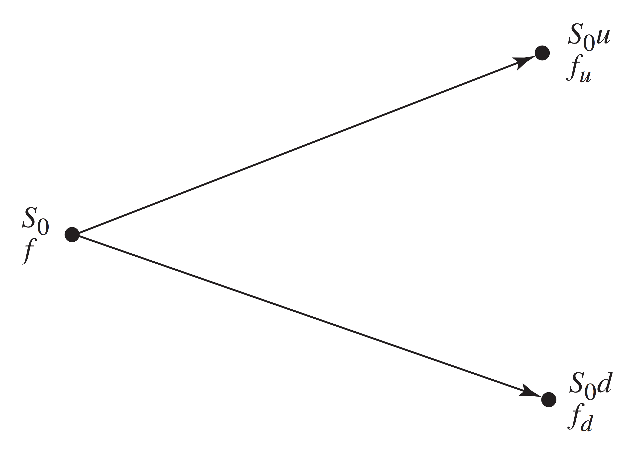
\[\begin{split}\begin{align} 5 - f & = 4.367 \\ \Rightarrow f & = 0.633. \end{align}\end{split}\]

One-Step Binomial Tree¶

We can generalize the previous example.

The current stock price is $\smash{S_0}$.

The current option price is $\smash{f}$.

Time periods are $\smash{T}$ years.

At the end of the next time period, the stock price will be either $\smash{S_0 u}$ or $\smash{S_0 d}$, where $\smash{u > 1}$ and $\smash{d < 1}$.

$\smash{u-1}$ represents a percentage increase and $\smash{d - 1}$ represents a percentage decrease.

The option values at the end of next time period are either $\smash{f_u}$ or $\smash{f_d}$.

One-Step Binomial Tree¶

One-Step Portfolio¶

Consider a portfolio that is long $\smash{\Delta}$ shares and short 1 call option.

If the stock price moves up, the value is $\smash{S_0 u \Delta - f_u}$.

If the stock price moves down, the value is $\smash{S_0 d \Delta - f_d}$.

Find $\smash{\Delta}$ such that the payoffs are equal:

\[\begin{split}\begin{align} \Delta & = \frac{f_u - f_d}{S_0 u - S_0 d}. \end{align}\end{split}\]

One-Step Portfolio¶

Since the payoffs are equivalent in each state, the portfolio is riskless.

Suppose the continuously compounded risk-free rate is $\smash{r}$.

The present value of the portfolio payoff is $\smash{\left(S_0 u \Delta - f_u\right) e^{-rT}}$.

The current cost of the portfolio is $\smash{S_0 \Delta - f}$.

Call Option Price¶

Equating cost and value of the portfolio:

\[\begin{split}\begin{align} S_0 \Delta - f & = \left(S_0 u \Delta - f_u\right) e^{-rT} \\ \Rightarrow f & = S_0 \Delta \left(1-u e^{-rT}\right) + f_u e^{-rT} \\ & = S_0 \frac{f_u-f_d}{S_0 u - S_0 d} \left(1-u e^{-rT}\right) + f_u e^{-rT} \\ & = \frac{f_u\left(1-d e^{-rT}\right) + f_d\left(u e^{-rT} - 1\right)}{u-d} \\ & = e^{-rT} \left(p f_u + (1-p) f_d\right), \end{align}\end{split}\]

where $\smash{p = \frac{e^{rT} - d}{u-d}}$.

Revisiting One-Period Example¶

Recall the previous example:

$\smash{u = 1.1}$, $\smash{d = 0.9}$, $\smash{f_u = 1}$, $\smash{f_d = 0}$, $\smash{r = 0.12}$ and $\smash{T = 3/12}$.

Thus $\smash{p = \frac{e^{0.12\times 3/12} - 0.9}{1.1-0.9} = 0.6523}$.

$\smash{f = e^{-0.12 \times 0.25} \left(0.6523 \times 1 + 0.3477 \times 0\right) = 0.633}$.

Two-Step Binomial Tree¶

Consider a two-period example, where the stock price can move up or down during the first period, and then can move up or down during the second period.

There will be either three or four possible stock prices at the end of time two.

We can solve the problem backwards:
- First solve for the prices of the options in each state of the world at the end of period 1 (two separate problems).
- Use those prices to solve for the price at the current time (single problem).

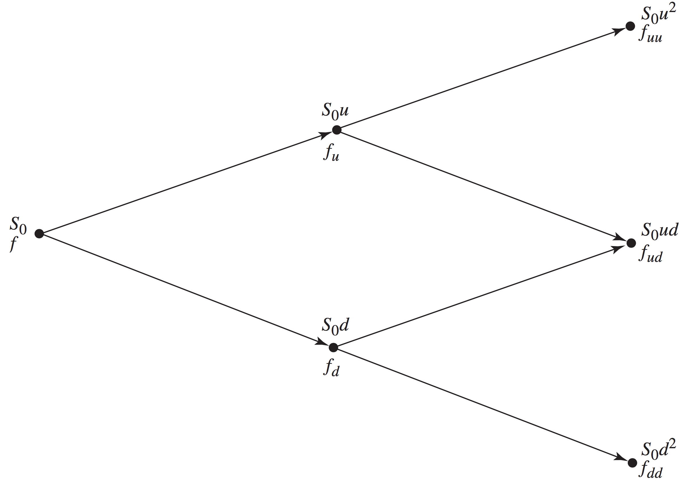
Two-Step Binomial Tree¶

Let us now denote a time period as $\smash{\Delta t}$.

The value (price) of the call option at the end of the first period in the high state is:

\[\begin{split}\begin{align} f_u & = e^{-r \Delta t} \left(p f_{uu} + (1-p) f_{ud}\right) \end{align}\end{split}\]

The value (price) of the call option at the end of the first period in the low state is:

\[\begin{split}\begin{align} f_d & = e^{-r \Delta t} \left(p f_{ud} + (1-p) f_{dd}\right) \end{align}\end{split}\]

Two-Step Binomial Tree¶

The value (price) of the call option at the current time is:

\[\begin{split}\begin{align} f & = e^{-r \Delta t} \left(p f_{u} + (1-p) f_{d}\right) \\ & = e^{-2r \Delta t}\left(p^2 f_{uu} + 2*p(1-p) f_{ud} + (1-p)^2 f_{dd} \right). \end{align}\end{split}\]

Two-Step Binomial Tree Example¶

Continuing with the previous example: $\smash{u = 1.1}$, $\smash{d = 0.9}$, $\smash{r = 0.12}$ and $\smash{\Delta t = 3/12}$.

If the stock price moves up twice $\smash{S_0 u^2 = 24.2}$ and $\smash{f_{uu} = 3.2}$.

If the stock price moves down twice $\smash{S_0 d^2 = 16.2}$ and $\smash{f_{dd} = 0}$.

If the stock price moves up and down $\smash{S_0 ud = 19.8}$ and $\smash{f_{ud} = 0}$.

Two-Step Binomial Tree Example¶

Given the numbers above:

\[\begin{split}\begin{align} f_u & = e^{-0.12 \times 0.25} \left(0.6523 \times 3.2 + 0.3477 \times 0 \right) = 2.0257 \\ f_d & = e^{-0.12 \times 0.25} \left(0.6523 \times 0 + 0.3477 \times 0 \right) = 0 \\ f & = e^{-0.12 \times 0.25} \left(0.6523 \times 2.0257 + 0.3477 \times 0 \right) = 1.2823. \end{align}\end{split}\]

Valuing Put Options¶

The foregoing treatment was not unique to call options.

We likewise could have determine the number of shares necessary to create a riskless portfolio that is long the stock and short a put.

This would result in a symmetric solution for $\smash{\Delta}$, but using the final values of the put in each state.

The same formulas for the one- and two-period trees can be used to value the option.
- The only difference is that the option payoffs at each node are different than the call.

Two-Step Put Option Example¶

The current price of a stock is $\smash{S_0 = \$50}$, $\smash{u = 1.2}$, $\smash{d = 0.8}$, $\smash{r = 0.05}$ and $\smash{\Delta t = 1}$. Consider a put with strike price $\smash{\$52}$.

If the stock price moves up twice $\smash{S_0 u^2 = 72}$ and $\smash{f_{uu} = 0}$.

If the stock price moves down twice $\smash{S_0 d^2 = 32}$ and $\smash{f_{dd} = 20}$.

If the stock price moves up and down $\smash{S_0 ud = 48}$ and $\smash{f_{ud} = 4}$.

$\smash{p = \frac{e^{r \Delta t} - d}{u-d} = \frac{e^{0.05 \times 1} - 0.8}{1.2-0.8} = 0.6282}$.

Two-Step Put Option Example¶

Given the numbers above:

\[\begin{split}\begin{align} f_u & = e^{-0.05 \times 1} \left(0.6282 \times 0 + 0.3718 \times 4 \right) = 1.4147 \\ f_d & = e^{-0.05 \times 1} \left(0.6282 \times 4 + 0.3718 \times 20 \right) = 9.4635 \\ f & = e^{-0.05 \times 1} \left(0.6282 \times 1.4147 + 0.3718 \times 9.4635 \right) = 4.1923. \end{align}\end{split}\]

American Options¶

To value an American option with a binomial tree:

At each node, compute the value of the call implied by the subsequent nodes (using the foregoing methods).

Compute the value of immediate exercise.

Assign the value as the maximum of these two quantities.

Proceed in reverse fashion until the value is computed at the first node, taking into account the possibilities of early exercise.

American Option Example¶

Suppose that the put in the previous example is an American option.

If the stock price moves down, the value of immediate exercise is $\smash{\$12}$.

This means $\smash{f_d = \max(9.4626,12) = 12}$.

As a result:

\[\begin{split}\begin{align} f & = e^{-0.05 \times 1} \left(0.6282 \times 1.4147 + 0.3718 \times 12 \right) = 5.0894. \end{align}\end{split}\]

Note that the value of the American option is greater than that of the European option.

Delta¶

Recall that $\smash{\Delta}$ is the number of shares that must be purchased to create a riskless portfolio with a short option.

It is the ratio of possible option values over the possible stock prices.

It is often written and referred to as delta.

Following this investment strategy is called delta hedging.

Call option deltas are positive and put option deltas are negative.

Call Deltas¶

In the two-period call option example:

\[\begin{split}\begin{align} \Delta_0 & = \frac{2.0257 - 0}{22-18} = 0.5064 \\ \Delta_u & = \frac{3.2 - 0}{24.2-19.8} = 0.7273 \\ \Delta_d & = \frac{0 - 0}{19.8-16.2} = 0, \end{align}\end{split}\]

where $\smash{\Delta_0}$ is the delta for the first time period and $\smash{\Delta_u}$ and $\smash{\Delta_d}$ are the deltas for the second periods if the price moves up and down.

Notice that delta changes with time - i.e you need to rebalance your portfolio to maintain a riskless hedge.

This is called dynamic hedging.

Put Deltas¶

In the two-period put option example:

\[\begin{split}\begin{align} \Delta_0 & = \frac{1.4147 - 9.4636}{60-40} = -0.4024 \\ \Delta_u & = \frac{0-4}{72-48} = -0.1667 \\ \Delta_d & = \frac{4-20}{48-32} = -1. \end{align}\end{split}\]

Stock Return Volatility¶

Suppose $\smash{\sigma^2}$ is the annualized variance of the stock returns.

Assuming the returns are independent, $\smash{\Delta t \sigma^2}$ is a good approximation of the variance for period $\smash{\Delta t}$.

This means a good approximation of the standard deviation, or volatility, for period $\smash{\Delta t}$ is $\smash{\sqrt{\Delta t} \sigma}$.

Binomial Tree Parameters¶

Given the current stock price, $\smash{S_0}$, the option strike price and the risk-free rate, $\smash{r}$:

The binomial tree is completely determined by three parameters: $\smash{u}$, $\smash{d}$ and $\smash{\Delta t}$.

$\smash{u}$ and $\smash{d}$ are often set so that $\smash{u = e^{\sigma \sqrt{\Delta t}}}$ and $\smash{d = e^{-\sigma \sqrt{\Delta t}}}$.

In doing so, it can be shown that the volatility of the returns in the binomial tree approximate $\smash{\sigma}$.

Binomial Tree Parameters¶

Simple binomial tree models with long time periods are unrealistic.

We can simply increase the number of steps in the model.

For example, for a three-month period with daily time steps, there would be a total of roughly 66 period (22 trading days per month).

For the recombining trees we considered above, this amounts to 66 possible terminal values and $\smash{\sum_{i=1}^{65} i = 2145}$ individual options nodes to value.

For the non-recombining trees, this amounts to $\smash{2^{65}}$ possible terminal values and $\smash{\sum_{i=1}^{65} 2^{i-1}}$ individual options nodes to value.

Options on Other Assets¶

We have only valued options on a stock that doesn’t pay dividends.

To value other assets, we only need to adjust the interest rate $\smash{r}$ used in the calculation of $\smash{p}$ to account for any earnings or costs associated with the underlying asset.

Discounting to present value is always done with $\smash{r}$.

Options on Other Assets¶

For stock paying dividends:

\[\begin{split}\begin{align} p & = \frac{e^{(r-q)\Delta t}-d}{u-d}. \end{align}\end{split}\]

For currencies:

\[\begin{split}\begin{align} p & = \frac{e^{(r-r_f)\Delta t}-d}{u-d}. \end{align}\end{split}\]

For futures:

\[\begin{split}\begin{align} p & = \frac{1-d}{u-d}. \end{align}\end{split}\]