The Term Structure of Interest Rates
Yield Curve
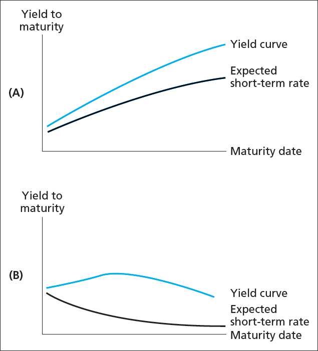
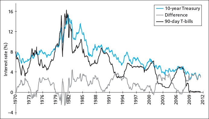
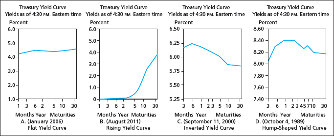
Bonds of different maturities often have different yields to maturity.
- The relationship between yield and maturity is summarized graphically in the yield curve.
- Consider several examples below.
\(\qquad\)
Yield Curve Slope
An upward sloping yield curve is evidence that short-term interest rates are going to rise.
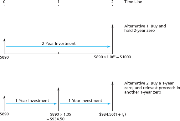
Consider two investment strategies.
- Buy and hold a two-year zero-coupon bond, offering 6% return each year.
- Buy a one-year bond today, offering a 5% return over the coming year, and roll the investment into another one-year zero-coupon bond a year from now, offering an interest rate of \(r_2\).
- These investments should be equivalent. Why?
Yield Curve Slope
Suppose you begin with $890 to invest (the price of a two-year zero-coupon bond with 6% YTM.
- Equating the returns to each strategy gives:
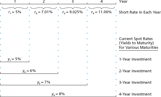
Spot Rates and Short Rates
We distinguish between two types of interest rates.
- Spot rate: the rate offered today on zero-coupon bonds of
different maturities.
- In the previous example, the one-year spot rate is 5% and the two year spot rate is 6%.
- Short rate: the rate for given time interval (one year) offered at
different points in time.
- In the previous example, the first-year short rate is 5% (same as the spot!) and the second-year short rate is 7.01%.
Spot Rates and Short Rates
The spot rate for a given period should be the geometric average of short rates over that interval.
- Let \(y_2\) be the two-year spot rate.
- Let \(r_1\) and \(r_2\) be the first-year and second-year short rates.
- Don’t forget that \(y_1 = r_1\).
Spot Rates and Short Rates
So, if the yield curve slopes up (\(y_2 > y_1 = r_1\)), we conclude that short-term rates will rise (\(r_2 > r_1\)).
- Reverse reasoning holds for a downward sloping yield curve.
Spot Rate and Short Rate Example
Assume the following spot rates and short rates:
- Spots: \(y_1 = 0.05\), \(y_2 = 0.06\) and \(y_3 = 0.07\).
- Shorts: \(r_1 = y_1\) and \(r_2 = 0.0701\).
- What is the three-year short rate, \(r_3\)?
Spot Rate and Short Rate Example
Buying a three-year zero-coupon bond should be identical to buying a two-year zero and rolling into a one-year zero.
Spot Rate and Short Rate Example
We know
So the full decomposition is
General Short Rates
We can generalize the previous results.
- Investing in an \(n\) period zero-coupon bond should be the same as investing in an \(n-1\) zero and rolling into a one-period zero at time \(n-1\).
Forward Rates
In the development above, we assumed no uncertainty.
- All future rates were known at time zero.
- In reality, we don’t have perfect knowledge of time \(n\) short rates at time zero.
Forward Rates
To distinguish between actual short rates that occur in the future, we define the forward rate to be
- The time \(t=n\) forward rate is the break-even interest rate that equates the returns of an n-period zero-coupon bond with an \((n-1)\) -period zero rolled into a one-period zero.
- It may not be equal to the expected future short rate.
Expectations Hypothesis
The Expectations Hypothesis of the yield curve says that expected short rates equal forward rates:
- If the yield curve slopes upward, short rates are expected to rise: \(E[r_n] > E[r_{n-1}] > r_1 = y_1\).
- If the yield curve slopes downward, short rates are expected to fall: \(E[r_n] < E[r_{n-1}] < r_1 = y_1\).
Liquidity Preference Theory
According to the Liquidity Preference Theory of the yield curve, investors must be compensated for holding longer-term bonds.
- Longer-term bonds are subject to greater risk, and so investors should demand a premium for holding them.
- In reality, a premium means that investors will only buy them for a lower price (which means greater yield).
Liquidity Preference Theory
The Liquidity Preference Theory can be expressed as forward rates being equal to expected short rates plus a premium, \(\phi\):
- According to this theory, expected short rates can be constant if the yield curve is upward sloping.
- If the yield curve is downward sloping, expected short rates must be falling. Why?
Liquidity Preference Example
Suppose you buy a two-year bond and that
- Short rates for the next two years are constant at 8%: \(r_1 = E[r_2] = 0.08\).
- The liquidity premium for year two is 1%: \(\phi = 0.01\).
Liquidity Preference Example
What is the yield to maturity of the two year bond?
- So the yield curve slopes up (\(y_2 > y_1\)) even though expected short rates are constant.
Expectations Hypothesis Example
However, if there is no liquidity premium
- Now the yield curve is flat.
Implications of the Theories
The slope of the yield curve always determines whether forward rates are rising or falling.
- \(y_2 > y_1\) means \(f_2 > f_1\) (by the definition of forward rates!).
- If the Expectations Hypothesis holds, \(E[r_2] = f_2\), so \(y_2 > y_1\) means \(E[r_2] > r_1 = f_1 = y_1\).
Implications of the Theories
If the Liquidity Preference Theory holds, we have no guarantee that \(E[r_2] > r_1\) if \(y_2 > y_1\).
- Short rates could be constant with a moderate liquidity premium.
- Short rates could be rising some, with a small liquidity premium.
- Short rates could be falling, with a large liquidity premium.
- What about if \(y_2 < y_1\)?