Index Models¶

Motivation¶

Recall that for portfolio optimization with \(N\) assets we must estimate all means, variances and covariances:

\[\begin{split}\# \,\, \text{of estimates} & = \frac{N(N+3)}{2}.\end{split}\]

Suppose you have a dataset consisting of 5 years of monthly returns for each asset (i.e. 60 observations per asset):

\(N\)	50	100	1000	3000
# Estimates	1325	5150	501,500	4,504,500
Data	3000	6000	60,000	180,000

Note: it is impossible to estimate \(P\) parameters with \(N\) data observations if \(N < P\).

Motivation¶

The return to an asset can always be decomposed into two parts:

\[\begin{split}r_i & = E[r_i] + \epsilon_i = \mu_i + \epsilon_i,\end{split}\]

where \(\epsilon_i\) has zero mean (\(\mu_{\epsilon_i} = 0\)) and standard deviation \(\sigma_{\epsilon_i}\).

The first term of the equation above is the expected return.

The second term is the unexpected, or unanticipated return (also referred to as a shock).

This decomposition is not dependent on a model or special assumptions.

Single-Factor Model¶

Suppose there is a market factor \(m\) that influences the returns to all firms.

Assume we can further decompose the shock, \(\epsilon_i\), into two parts:

\[\epsilon_i = \beta_i m + \varepsilon_i.\]

Single-Factor Model¶

In this case the return can be written as a single-factor model:

(1)\[\begin{split}r_i & = \mu_i + \beta_i m + \varepsilon_i.\end{split}\]

\(m\) and \(\varepsilon_i\) have means \(\mu_m = \mu_{\varepsilon_i} = 0\), standard deviations \(\sigma_m\) and \(\sigma_{\varepsilon_i}\), and are uncorrelated (\(Cov(m, \varepsilon_i) = 0\)).

\(\epsilon_i\) is still unanticipated since \(\mu_{\epsilon_i} = \mu_m + \mu_{\varepsilon_i} = 0\).

\(\beta_i\) is a measure of the sensitivity of \(r_i\) to \(m\).

Decomposing Risk¶

We can now compute variances using the model:

\[\begin{split}\sigma^2_i & \equiv Var(r_i) = Var(\mu_i + \beta_i m + \varepsilon_i) \qquad\end{split}\]

\[\begin{split}& \qquad = \beta^2_i Var(m) + Var(\varepsilon_i) + 2\beta_iCov(m,\varepsilon_i)\end{split}\]

\[\begin{split}& = \beta^2_i \sigma^2_m + \sigma^2_{\varepsilon_i}. \qquad \qquad \qquad \quad \,\end{split}\]

We made use of \(Var(\mu_i) = 0\) and \(Cov(m,\varepsilon_i) = 0\).

\(Var(r_i)\) arises from two separate sources.
- \(\beta^2_i \sigma^2_m\): risk due to \(m\). Since this is common to all assets, it is the systematic component.
- \(\sigma^2_{\varepsilon_i}\): idiosyncratic component specific to each asset.

Decomposing Risk¶

We can use the model to compute covariances between assets:

\[\begin{split}Cov(r_i,r_j) & = Cov(\mu_i + \beta_i m + \varepsilon_i, \mu_j + \beta_j m + \varepsilon_j)\end{split}\]

\[\begin{split}& = \beta_i \beta_j Cov(m,m) \qquad \quad\end{split}\]

\[\begin{split}& = \beta_i \beta_j \sigma^2_m. \qquad \qquad \quad \enspace\end{split}\]

\(Var(\mu_i) = Var(\mu_j) = Cov(\mu_i,\mu_j) = 0\), since \(\mu_i\) and \(\mu_j\) are constants.

We assumed \(Cov(\varepsilon_i, \varepsilon_j) = 0\).

Intuitively, unanticipated shocks to different assets shouldn’t be correlated.

Using an Index as a Factor¶

So what is \(m\)?

We would like to find a macroeconomic variable correlated with all assets.

It is common to use a market index portfolio, such as the S&P 500 (we expect the return of a broad index to be correlated with individual assets).

Using an Index as a Factor¶

In particular, let’s use \(m = r_m - \mu_m\), where \(r_m\) is the return to the S&P 500 (\(m\) stands for market).

In this case

\[\begin{split}E[m] & = E[r_m - \mu_m] \quad\end{split}\]

\[\begin{split}& \quad = E[r_m] - \mu_m \,\end{split}\]

\[\begin{split}& = \mu_m - \mu_m \,\end{split}\]

\[\begin{split}& = 0. \qquad \enspace\end{split}\]

So our assumption of \(E[m] = 0\) is satisfied.

Single-Index Model¶

Substituting this factor into the single-factor model of Equation (1):

\[\begin{split}r_i & = \mu_i + \beta_i (r_m - \mu_m) + \varepsilon_i.\end{split}\]

We then manipulate the equation:

\[\begin{split}r_i & = r_f - r_f + \mu_i + \beta_i(r_m - r_f + r_f - \mu_m) + \varepsilon_i \qquad \quad\end{split}\]

\[\begin{split}& = r_f + \underbrace{(\mu_i - r_f) - \beta_i (\mu_m - r_f)}_{\alpha_i} + \beta_i (r_m - r_f) + \varepsilon_i \,\end{split}\]

(2)\[\Rightarrow r_{i,e} = \alpha_i + \beta_i r_{m,i} + \varepsilon_i.\]

Single-Index Model¶

Equation (2) is the single-index model.

Note: \(\alpha_i = rp_i - \beta_i rp_m\).

Expected Return-Beta Relationship¶

Taking expectations of Equation (2), we find

\[\begin{split}rp_i & = \alpha_i + \beta_i rp_m,\end{split}\]

since \(E[\varepsilon_i] = 0\).

\(\beta_i\) is known as the security Beta and is a measure of the sensitivity of asset \(i\) to the market index.

\(\beta_i rp_m\) is the systematic risk premium, since it is the premium one could expect for taking on systematic risk.

\(\alpha_i\) is the non-market premium. It is the risk premium expected above that provided by the market.

In equilibrium we expect \(\alpha_i = 0\).

Why \(\alpha\) Must Be Zero¶

Why do we expect \(\alpha_i = 0\)?

Suppose \(\alpha_i > 0\).

We expect individuals to buy more of asset \(i\), putting more weight on it in their individual portfolios relative to the market portfolio.

If everyone did this, the market portfolio would put higher weight on asset \(i\).
- Everyone deviates from the market portfolio by holding more of asset \(i\).
- But since everyone constitutes the market, the market portfolio shifts by the exact amount that they want to hold asset \(i\).

Single-Index Regression¶

We express the single-index model as a regression:

\[\begin{split}r_{i,e}(t) & = \alpha_i + \beta_i r_{m,e}(t) + \varepsilon_i(t),\end{split}\]

where the \(t\) denotes that the relationship must hold for all observations through time.

We estimate the model by collecting historical observations for \(r_m\), \(r_i\) and \(r_f\) and then computing the regression estimates for \(\alpha_i\) and \(\beta_i\).

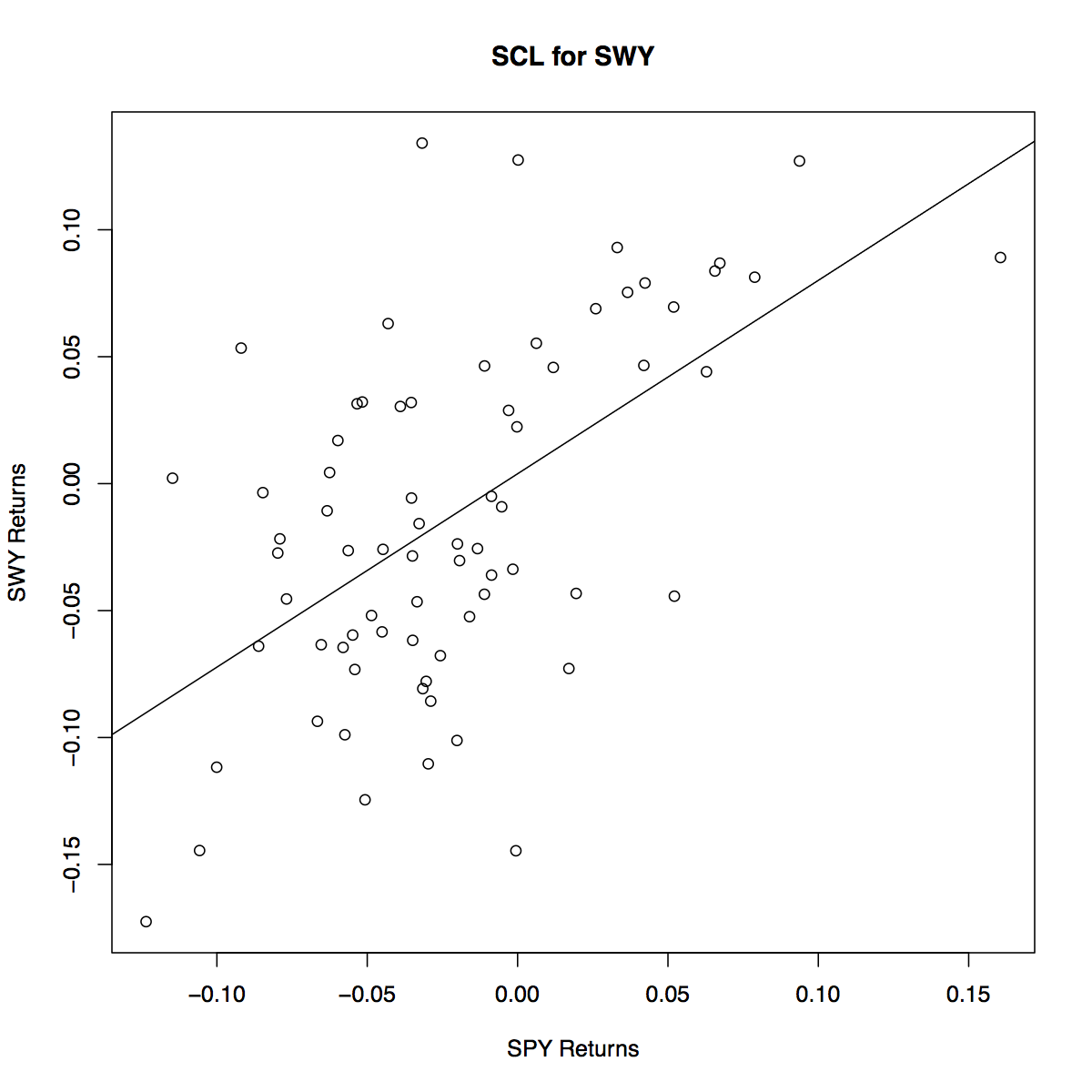
Security Characteristic Line¶

The regression estimates of \(\alpha_i\) and \(\beta_i\) are denoted by \(\hat{\alpha}_i\) and \(\hat{\beta}_i\).

The fitted values of the regression are

(3)\[\begin{split}\hat{r}_{i,e}(t) & = \hat{\alpha}_i + \hat{\beta}_i r_{m,e}(t).\end{split}\]

\(\hat{r}_{i,e}(t)\) are the values of the regression line.

They are the values we expect \(r_{i,e}\) to take for given values of \(r_{m,e}\).

Security Characteristic Line¶

Residuals are not included since they are unexpected (deviations from the line).

Equation (3) is known as the Security Characteristic Line or SCL.

Advantages of the Model¶

Suppose we want to use the Index Model to produce the estimates required for portfolio optimization.

Assume there are \(N\) assets in the portfolio.

From the model,

\[\begin{split}\mu_{i,e} & = \alpha_i + \beta_i \mu_{m,e}\end{split}\]

\[\begin{split}\sigma^2_i & = \beta^2_i \sigma^2_m + \sigma^2_{\varepsilon_i}\end{split}\]

and

\[\begin{split}\sigma_{ij} & = \beta_i \beta_j \sigma^2_m.\end{split}\]

Advantages of the Model¶

Let’s count the number of parameters we must estimate.

\(N\) estimates of \(\alpha_i\).

\(N\) estimates of \(\beta_i\).

\(N\) estimates of \(\sigma^2_{\varepsilon_i}\).

One estimate of \(\mu_m\).

One estimate of \(\sigma_m\).

Advantages of the Model¶

That’s a total of \(3N+2\) estimates.

We’ll see this is much better than \(\frac{N(N+3)}{2}\) estimates without the model.

Advantages of the Model¶

Suppose you have a dataset consisting of 5 years of monthly returns for each asset (i.e. 60 observations per asset):

\(N\)	50	100	1000	3000
# Estimates No Model	1325	5150	501,500	4,504,500
# Estimates Index Model	152	302	3002	9002
Data	3000	6000	60,000	180,000

Clearly estimation is much more reasonable with the single-index model for large \(N\).

Cost of the Model¶

The index model restricts the relationship among the asset variances and covariances to be of a specific form.

It is precisely this imposed structure that relieves us of the estimation burden.

However, it oversimplifies the true nature of the world.

For example, it dichotomizes security risk into two components: market and asset specific.

But neglects to account for industry specific risk, etc.

In this sense, the model may fail to capture important aspects of market.

Index Model Portfolios¶

Suppose you hold a portfolio of \(N\) assets with weights \(\omega_i\), \(i=1,\ldots,N\).

Then

\[\begin{split}r_{p,e} & = \sum_{i=1}^N \omega_i r_{i,e} = \sum_{i=1}^N \omega_i (\alpha_i + \beta_i r_{m,e} + \varepsilon_i) \qquad\end{split}\]

\[\begin{split}& \,= \underbrace{\sum_{i=1}^N \omega_i \alpha_i}_{\alpha_p} + \underbrace{\left(\sum_{i=1}^N \omega_i \beta_i \right)}_{\beta_p} r_{m,e} + \underbrace{\sum_{i=1}^N \omega_i \varepsilon_i}_{\varepsilon_p}\end{split}\]

\[\begin{split}& = \alpha_p + \beta_p r_{m,e} + \varepsilon_p. \qquad \qquad \qquad \quad\end{split}\]

Index Model Portfolio Coefficients¶

The mathematics highlight some very nice results.

\(\alpha_p\): The non-market return of the portfolio is a weighted average of the non-market returns of individual assets.

\(\beta_p\): The sensitivity of the portfolio to the market excess return is a weighted average of the sensitivities of individual assets.

\(\varepsilon_p\): The portfolio shock is a weighted average of individual shocks.

Index Model Portfolio Risk¶

Since the portfolio is described by a single index model, its risk can be decomposed as

\[\begin{split}\sigma^2_p & = \beta^2_p \sigma^2_m + \sigma^2_{\varepsilon_p}.\end{split}\]

Note that,

\[\begin{split}\beta^2_p & = \left(\sum_{i=1}^N \omega_i \beta_i\right)^2\end{split}\]

not

\[\begin{split}\beta^2_p & = \sum_{i=1}^N \omega^2_i \beta^2_i.\end{split}\]

Index Model Portfolio Risk¶

The variance of \(\varepsilon_p\) can be written as

(4)\[\begin{split}\sigma^2_{\varepsilon_p} & \equiv Var(\varepsilon_p) = Var\left(\sum_{i=1}^N \omega_i \varepsilon_i \right)\end{split}\]

(5)\[\begin{split}& = \sum_{i=1}^N \omega^2_i Var(\varepsilon_i) \qquad \quad \enspace\end{split}\]

(6)\[\begin{split}& = \sum_{i=1}^N \omega^2_i \sigma^2_{\varepsilon_i} \qquad \qquad \quad\end{split}\]

Equation (5) follows from Equation (4) because we assume that \(Cov(\varepsilon_i, \varepsilon_j) = 0\) for \(i \neq j\).

Index Model Diversification¶

In the special case of an equally-weighted portfolio

\[\sigma^2_{\varepsilon_p} = \frac{1}{N^2} \sum_{i=1}^N \sigma^2_{\varepsilon_i} = \frac{1}{N} \overline{\sigma^2_{\varepsilon_p}},\]

where

\[\overline{\sigma^2_{\varepsilon_p}} = \frac{1}{N} \sum_{i=1}^N \sigma^2_{\varepsilon_i}.\]

Clearly,

\[\begin{split}\lim_{N \to \infty} \overline{\sigma^2_{\varepsilon_p}} & = 0.\end{split}\]

Index Model Diversification¶

Recall

\[\begin{split}\sigma^2_p & = \beta^2_p \sigma^2_m + \sigma^2_{\varepsilon_p}.\end{split}\]

Thus,

\[\begin{split}\lim_{N \to \infty} \sigma^2_p & = \lim_{N \to \infty} \beta^2_p \sigma^2_m + \lim_{N \to \infty} \sigma^2_{\varepsilon_p}\end{split}\]

\[\begin{split}& = \beta^2_p \sigma^2_m.\end{split}\]

Index Model Diversification¶

\(\qquad\)

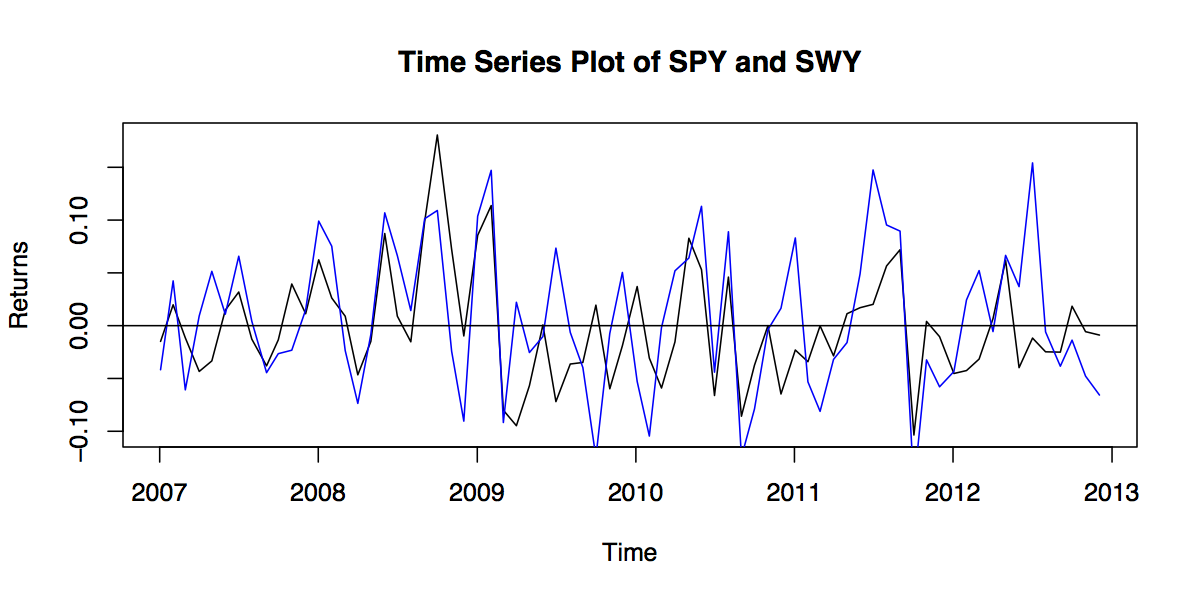
Index Model Example¶

Let’s estimate an index model.

Use SPY (S&P 500 SPDR) as a surrogate for market returns.

Estimate the model for SWY (Safeway).

Download 5 years of monthly data from Yahoo Finance, between 1 Jan 2007 and 31 Dec 2012.

Use adjusted closing prices to compute returns.

Estimate the regression.

Index Model Example¶

\(\qquad\)

Index Model Example¶

Parameter	Estimate	Standard Error	P-Value
\(\alpha\)	0.003903	0.007387	0.599
\(\beta\)	0.7620	0.1319	1.92e-07

The Adjusted \(R^2\) is 0.3133.