Asset Allocation
Utility
Investors usually care about maximizing utility.
- Suppose all investors have utility function
- \(\mu\) and \(\sigma\) are the mean and standard deviation of asset returns.
- What is the utility of holding a risk-free asset \(U(\mu_f, \sigma_f)\)?
Certainty Equivalent
For a risky portfolio, \(U(\mu_f, \sigma_f)\) can be thought of as a certainty equivalent return.
- The return that a risk-free asset would have to offer to provide the same utility level as a risky asset.
Risk Aversion
The parameter \(\gamma\) is a measure of risk preference.
- If \(\gamma > 0\) individuals are risk averse - volatility detracts from utility.
- If \(\gamma = 0\) individuals are risk neutral - volatility
doesn’t enter into the utility function.
- In this case, investors rank portfolios by their expected return and don’t care about portfolio riskiness.
Risk Aversion
- If \(\gamma < 0\) individuals are risk lovers - volatility is
rewarded in the utility function.
- In this case, investors enjoy and get utility by taking on risk.
- We will generally assume investors are risk averse, with the magnitude of \(\gamma\) dictating the amount of risk aversion.
Mean-Variance Criterion
Under this utility model, investors prefer higher expected returns and lower volatility.
- Let portfolio \(A\) have mean and volatility \(\mu_A\) and \(\sigma_A\).
- Let portfolio \(B\) have mean and volatility \(\mu_B\) and \(\sigma_B\).
- If \(\mu_A \geq \mu_B\) and \(\sigma_A \leq \sigma_B\), then \(A\) is preferred to \(B\).
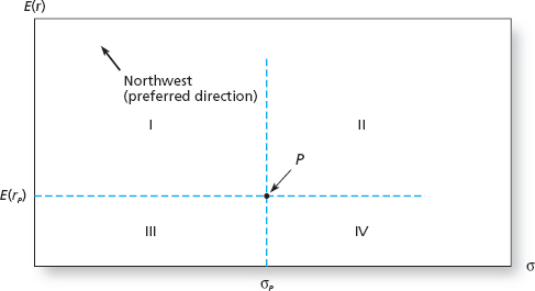
Indifference Curves
Portfolios in quadrant I are preferred to \(P\), which is preferred to portfolios in quadrant IV.
- What about quadrants II and III?
- If a portfolio \(Q\) has a mean and volatility that differ from \(P\) but yields the same utility level, then either
or
- That is, Q must be in quadrants II or III.
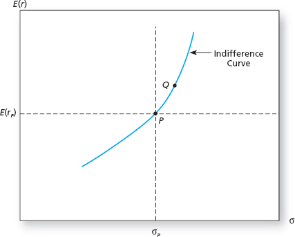
Indifference Curves
- The portfolios that yield the same utility as \(P\) constitute an indifference curve.
- We conclude that the indifference curve must cut through quadrants II and III.
Portfolios of Assets
Suppose an individual can invest in two assets: a risky portfolio \(P\) and a risk-free asset \(F\).
- \(\omega\) will be the fraction wealth invested in \(P\).
- \(1-\omega\) will be the fraction wealth invested in \(F\).
- We will typically assume that portfolio weights sum to 1.
- \(r_p\) will denote the return on asset \(P\), with \(\mu_p = E[r_p]\) and \(\sigma_p^2 = Var(r_p)\).
- \(r_f\) will denote the return on asset \(F\), with \(\mu_f = r_f\) and \(\sigma_f^2 = 0\).
Portfolio Return
Let \(C\) denote the portfolio that combines the two assets.
- \(C\) is a weighted average of \(P\) and \(F\):
- The return to \(C\), is
Portfolio Return
By the linearity of expectations:
- The term in the parentheses is the risk premium of \(P\).
Portfolio Volatility
According to the properties of variance,
- The third equality follows because \(r_f\) is a constant.
- Thus,
Portfolios and Risk Aversion
Portfolio \(C\) earns a base return of \(r_f\) plus the risk premium associated with \(P\), weighted by the amount of wealth the investor allocates to \(P\).
- More risk averse investors (small \(\omega\)) expect a rate of return closer to \(r_f\).
- Less risk averse investors (high \(\omega\)) expect a rate closer to \(\mu_p - r_f\).
- More risk averse investors have smaller portfolio volatilities.
- Less risk averse investors have higher portfolio volatilities.
Sharpe Ratio
Thus
- \(\text{SR}_p\) is the Sharpe Ratio of portfolio \(P\).
Capital Allocation Line
The Capital Allocation Line (CAL) depicts the set of portfolios available to an investor (a budget constraint).
- It plots pairs of \(\sigma_c\) and \(\mu_c\) that the investor can choose by selecting \(\omega\).
- This is simply a plot of the equation
- Clearly, the intercept will be \(r_f\) and the slope will be \(\text{SR}_p\).
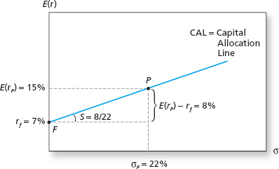
Capital Allocation Line Example
Suppose
- \(r_f = 0.07\).
- \(\mu_p = 0.15\).
- \(\sigma_p = 0.22\).
What is the CAL?
Simple Portfolio Choice
Individuals seek to maximize utility subject to the available choice set.
subject to
Simple Portfolio Choice (Cont.)
Substituting the constraints, the maximization problem becomes
Taking the derivative of this equation w.r.t. \(\omega\),
Simple Portfolio Choice
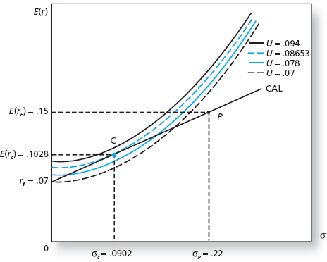
Since the CAL is a choice set (budget constraint), we can find the optimal portfolio by observing where an indifference curve is tangent to the CAL.
- Fix the utility value at \(\bar{U} = r_f\).
- Use the relation \(\bar{U} = \mu_c - \frac{1}{2} \gamma \sigma^2_c\) to solve for \(\mu_c\):
Simple Portfolio Choice
- Using this equation, we find the pairs of \(\mu_c\) and \(\sigma_c\) that corresponds to utility \(\bar{U}\), which we plot.
- Repeat this process, increasing the values of \(\bar{U}\) until a tangent indifference curve is found. The tangency corresponds to the optimal portfolio.
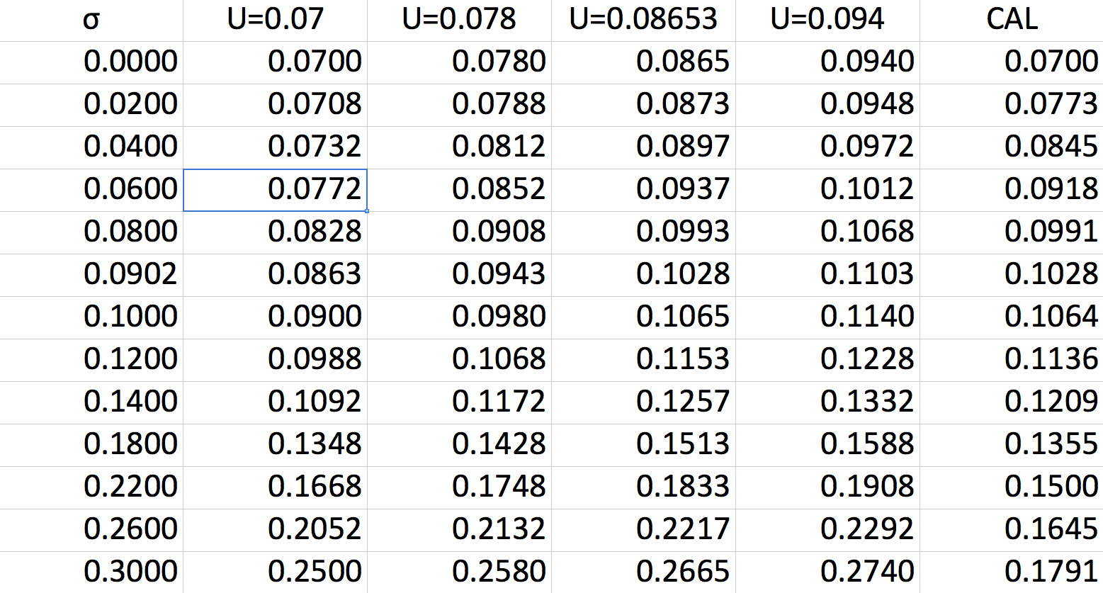
Spreadsheet Optimization
Given \(\gamma=2\), \(\mu=0.15\), \(\sigma=0.22\) and \(r_f=0.07\).
\(\qquad\)
Capital Market Line
Consider a value-weighted portfolio of all assets in the market.
- We will call this the market portfolio and denote it by \(M\).
- The CAL which connects \(r_f\) with \(M\) is called the Capital Market Line (CML).
- Because the true market portfolio is unobserved, we use a proxy - a well diversified portfolio that provides a good representation of the entire market.
- Typically we use the S&P 500.
Passive vs. Active Strategies
Holding the market portfolio or a market proxy is known as a passive strategy.
- It requires no security analysis.
- An active strategy is one that requires individual security analysis.