Risk and Risk Premiums¶

Probabilistic Returns¶

Since we don’t know future returns, we will treat them as random variables.

We can model them as discrete random variables, taking one of a finite set of possible values in the future: \(r(s)\), \(s = 1, \ldots, S\).
- In this case the probability of each value is \(p(s)\), \(s=1,\ldots,S\).

We can model them as continuous random variables, taking one of an infinite set of possible values in the future: \(r(s)\), \(s \in \mathcal{S}\) (e.g. \(\mathcal{S} = (-\infty, \infty)\)).
- In this case the probability of each value (kind of) is \(f(s)\), \(s \in \mathcal{S}\).

Expected Returns¶

Our best guess for the future return is the expected value:

\[\begin{split}E[r] & \equiv \mu = \sum_{s=1}^S r(s) p(s),\end{split}\]

or

\[\begin{split}E[r] & \equiv \mu = \int_{s \in \mathcal{S}} r(s) f(s) dr(s).\end{split}\]

Return Volatility¶

The amount of uncertainty in potential returns can be measured by the variance or standard deviation.

Volatility of returns specifically refers to standard deviation, NOT VARIANCE.

\[\begin{split}Std(r) & \equiv \sigma = \sqrt{\sum_{s=1}^S (r(s) - \mu)^2 p(s)},\end{split}\]

or

\[\begin{split}Std(r) & \equiv \sigma = \sqrt{\int_{s \in \mathcal{S}} (r(s) - \mu_r)^2 f(s) dr(s)}.\end{split}\]

Expectation and Variance Example¶

State	Probability	Return
Severe Recession	0.05	-0.37
Mild Recession	0.25	-0.11
Normal Growth	0.40	0.14
Boom	0.30	0.30

What are \(\mu\) and \(\sigma\)?

\[\begin{split}\mu & = 0.05*(-0.37) + 0.25*(-0.11) \\ & \qquad \qquad + 0.40*0.14 + 0.30*0.30 = 0.10\end{split}\]

\[\begin{split}E[r^2] & = 0.05*(-0.37)^2 + 0.25*(-0.11)^2 \\ & \qquad \qquad + 0.40*(0.14)^2 + 0.30*(0.30)^2 = 0.04471\end{split}\]

\[\begin{split}\sigma & = \sqrt{E[r^2] - \mu^2} = 0.04471 - 0.10^2 = 0.03471\end{split}\]

Assumption of Normality¶

It will often be convenient to assume asset returns are normally distributed.

In this case, we will treat returns as continuous random variables.

We can use the normal density function to compute probabilities of possible events.

We will not assume that returns of different assets come from the same normal, but instead FROM DIFFERENT normal distributions.

Differing Normal Distributions¶

As an example, suppose that

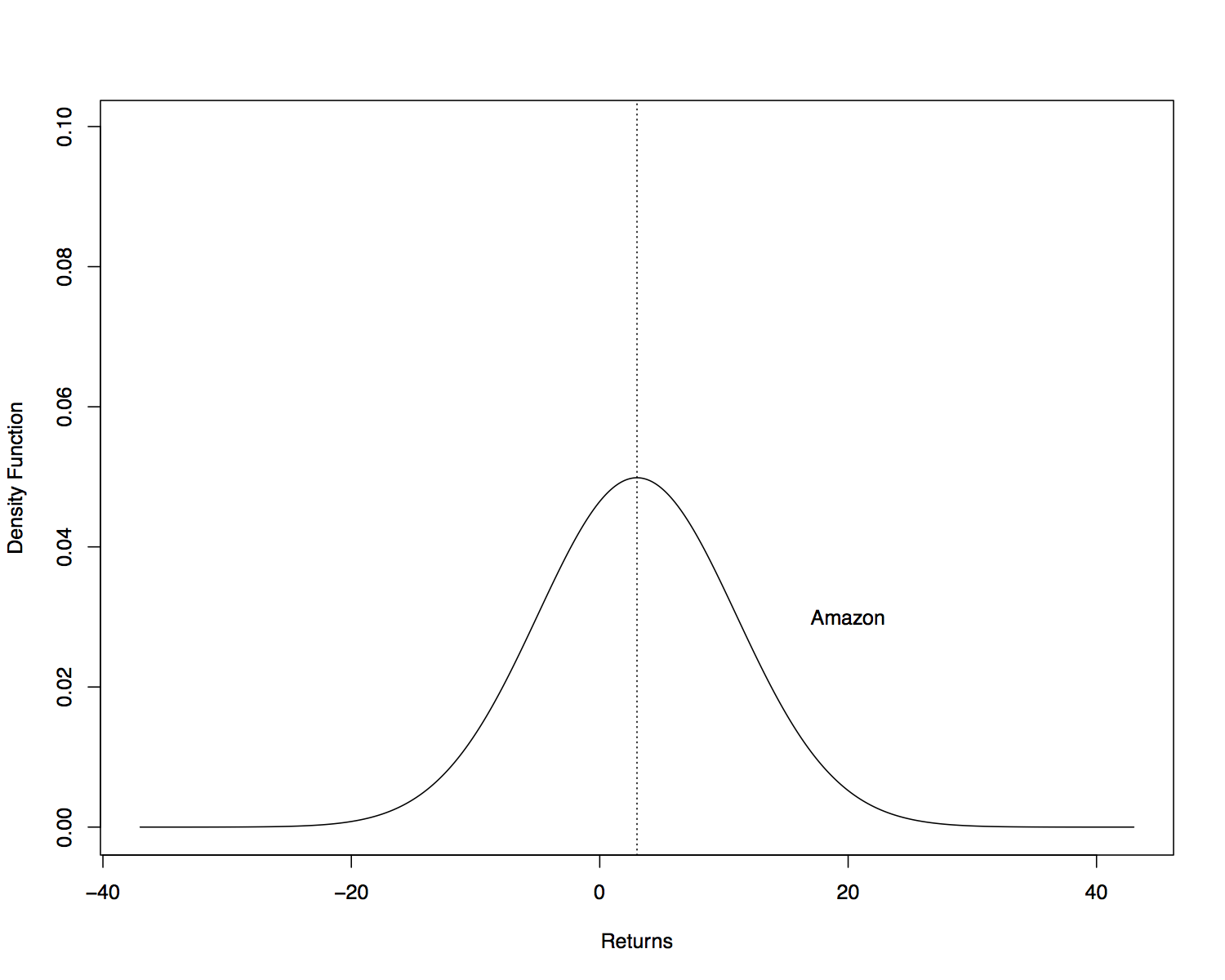
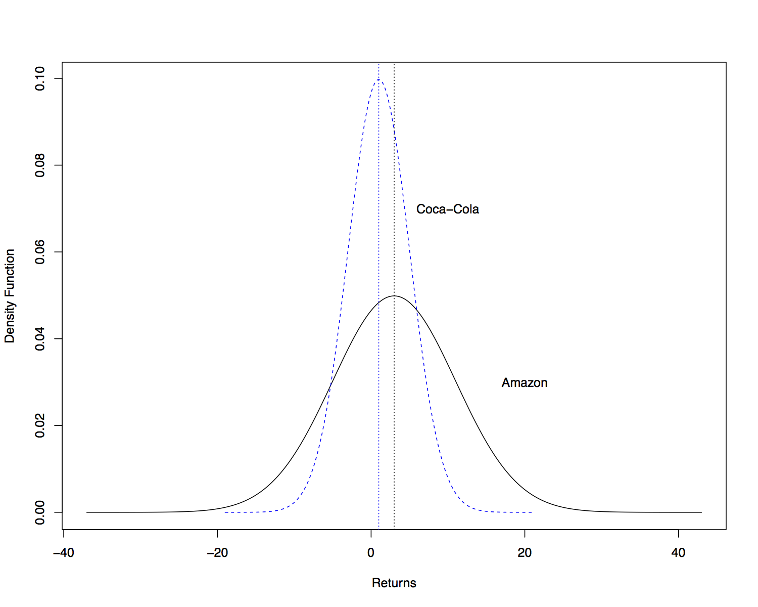
Amazon stock (AMZN) has an expected monthly return of 3% and a volatility (standard deviation) of 8%.

Coca-Cola stock (KO) has an expected monthly return of 1% and a volatility (standard deviation) of 4%.

What do their probability distributions look like?

Amazon Distribution¶

Coca-Cola Distribution¶

Implications of Normality¶

The assumption of normality is convenient because

If we form a portfolio of assets that are normally distributed, then the distribution of the portfolio return is also normally distributed.
- Recall that if \(X_i \sim \mathcal{N}(\mu_i, \sigma_i)\), \(i = 1,\ldots,N\), then \(W = \sum_{i=1}^N w_i X_i\) is also normally distributed (where \(w_i\) are constant weights).

The mean and the variance (or standard deviation) fully characterize the distribution of returns.

The variance or standard deviation alone is an appropriate measure of risk (no other measure is needed).

Estimating Means and Volatilities¶

Typically we don’t know the true mean and standard deviation of Amazon and Coca-Cola. What do we do?

Use historical data to estimate them.

Collect \(N+1\) past prices of each asset for a particular interval of time (daily, monthly, quarterly, annually).

Compute \(N\) returns using the formula

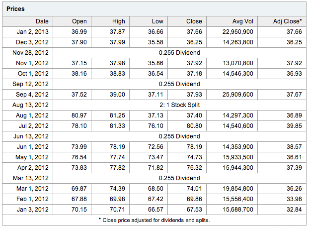
\[\begin{split}r_t & = \frac{P_t - P_{t-1}}{P_{t-1}}.\end{split}\]

We don’t include dividends in the return calculation above, because we use ADJUSTED closing prices, which account for dividend payments directly in the prices.

Estimating Means and Volatilities¶

Compute the sample mean of returns

\[\begin{split}\hat{\mu} & = \frac{1}{N} \sum_{t=1}^N r_t.\end{split}\]

Compute the sample standard deviation of returns

\[\begin{split}\hat{\sigma}^2 & = \frac{1}{N-1} \sum_{t=1}^N (r_t - \hat{\mu})^2.\end{split}\]

The “hats” indicate that we have estimated \(\mu\) and \(\sigma\): these are not the true, unknown values.

Estimating Means and Volatilities - Example¶

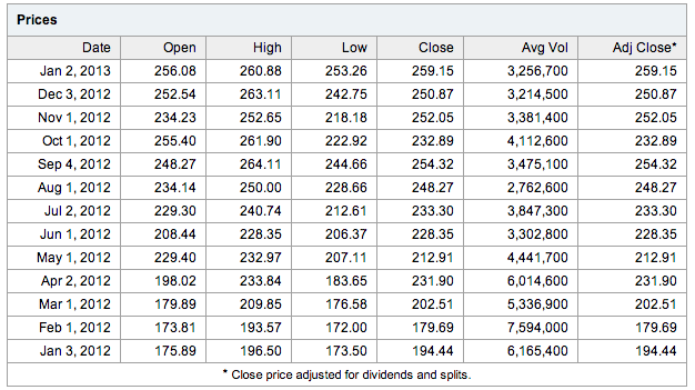
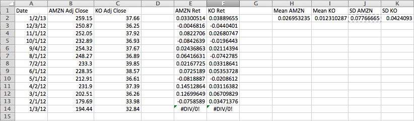
Let’s collect the \(N = 13\) closing prices for Amazon and Coca-Cola between 3 Jan 2012 and 2 Jan 2013.

We will only keep the first closing price on the first trading day of each month.

We can then compute 12 monthly returns by computing the difference in month prices at the beginning of each month, dividing by the price of the previous month.

This will give us 12 returns that we can use to estimate the means and standard deviations.

Amazon Monthly Prices¶

Coca-Cola Monthly Prices¶

Computing Returns and Moments¶

Risk-Free Returns¶

We will typically assume that a risk-free asset is available for purchase.

We will denote the risk-free return as \(r_f\).

If an asset is risk free, its return is certain and has no variability:

\[\begin{split}E[r_f] & = r_f \\ Var(r_f) & = 0.\end{split}\]

T-Bills as Risk-Free Assets¶

The return on a short-term government t-bill is usually considered risk free:

Although the price changes over time, the risk of default is extremely low.

Also, the holding period return can be determined at the beginning of the holding period (unlike other risky assets).

Compensation for Risk¶

If you can invest in a risk-free asset, why would you purchase a risky asset instead?

Risky assets compensate for risk through higher expected return.

If risky assets didn’t offer higher expected return, everyone would sell them, leading to a price decline today and a higher expected return:

\[\begin{split}\uparrow E[r_t] & = \frac{E[P_t] - \downarrow P_{t-1}}{\downarrow P_{t-1}}\end{split}\]

There is no guarantee that the actual return will be higher – only its expected value.

Risk Premium & Excess Returns¶

The amount by which the expected return of some risky asset \(A\) exceeds the risk-free return is known as the risk premium:

\[\begin{split}\text{rp}_{A,t} & = E[r_{A,t}] - r_{f,t}.\end{split}\]

The excess return measures the difference between a previously observed holding period return of \(A\) and the risk-free:

\[\begin{split}\text{er}_{A,t-1} & = r_{A,t-1} - r_{f,t-1}.\end{split}\]

Risk Premium & Excess Returns¶

Note that excess returns can only be computed with past returns.

We estimate risk premia with the sample mean of historical excess returns.

Sharpe Ratio¶

The Sharpe Ratio is a measure of how much risk premium investors require, per unit of risk:

\[\begin{split}\text{SR}_{A,t} & = \frac{\mu_{A,t} - r_{f,t}}{\sigma_{A,t}}\end{split}\]

The Sharpe Ratio is a measure of risk aversion.

It is often referred to as the price of risk.

The Sharpe Ratio for a broad market index of assets (like the S&P 500) is referred to as the market price of risk.

The true Sharpe Ratio is unknown, since we don’t know \(\mu_{A,t}\) and \(\sigma_{A,t}\), but we can estimate these with historical returns.

Risk Premium Example¶

Suppose the monthly risk-free rate is 0.2%. What is the estimated risk premium and Sharpe Ratio for Amazon stock?

\[rp_{AMZN} = 0.03 - 0.002 = 0.028\]

\[SR_{AMZN} = \frac{rp_{AMZN}}{0.08} = 0.35\]