Portfolio Optimization with Many Risky Assets
Portfolio Returns
Suppose you can now invest in an arbitrary number (\(N\)) of risky assets.
- Index the assets by \(i = 1, \ldots, N\).
- Let \(\omega_i\) be the fraction of income invested in asset \(i\).
- We will always assume that \(\sum_{i=1}^N \omega_i = 1\).
- We will denote the return to asset \(i\) by \(r_i\).
- The portfolio return is expressed as
Portfolio Moments
From the properties of expectation and variance, we can compute the mean and variance of the portfolio return.
- Recognize that the \(N\) asset returns, \(r_i\), are random variables.
- Denote the means of \(r_i\) as \(\mu_i\).
Portfolio Moments
- The \(N \times N\) covariance matrix of the returns contains the variances, \(\sigma^2_i\), and covariances, \(Cov(r_i, r_j) = \sigma_{ij}\):
Portfolio Moments
Thus resulting moments of the portfolio are
What are other ways to express \(\sigma^2_p\)?
Optimization: Risky MV Frontier
To determine the set of efficient risky portfolios (the risky frontier), the investor solves
subject to
where \(\mu_p\) is some prespecified value of the portfolio mean return.
Optimization: Risky MV Frontier
Note that
- The optimization problem has \(N-1\) choice variables: \(\{\omega_i\}_{i=1}^{N-1}\).
- \(\omega_N\) is not a choice variable because it is found from the constraint: \(\omega_N = 1 - \sum_{i=1}^{N-1} \omega_i\).
- This is a challenging problem that is only tractable with linear algebra (we won’t solve it).
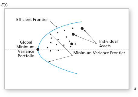
Risky Minimum-Variance Frontier
The frontier generated by multiple risky assets is known as the risky minimum-variance (MV) frontier.
- The lower portion of the frontier is inefficient since a higher mean portfolio exists with the same volatility on the upper portion of the frontier.
- The efficient MV frontier is generated by allowing investment in a risk-free asset and finding the CAL which is tangent to the risky efficient MV frontier.
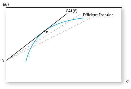
Optimization: Efficient MV Frontier
To determine the tangency portfolio, the investor solves the same problem as before
subject to
Optimization: Investor Choice
So far we have specified two optimization problems:
- To determine the risky minimum-variance frontier by minimizing variance subject to a particular expected return.
- To determine the tangency portfolio, by maximizing the Sharpe Ratio subject to constraints on the mean and standard deviation.
Neither of these made use of preferences. A final optimization problem would be the same as before:
- Maximize utility, \(U(\mu_p, \sigma_p)\), subject to investing in the tangency portfolio and a risk-free asset.
Estimation
In practice we must estimate \(\mu_i\), \(\sigma^2_i\) and \(\sigma_{ij}\) for \(i=1,\ldots,N\) and \(j=i+1,\ldots,N\).
- A total of \(N\) estimates of means.
- How many variances and covariances must we estimate?
- A total of \(N\) elements on the diagonal (variances).
- All of the elements above or below the diagonal (not both because of symmetry).
Estimation
- The resulting number of variance and covariance estimates is
Estimation
The total number of estimates is
- As an example, a portfolio of 50 stocks requires \(\frac{50 \times 53}{2} = 1325\) estimates.
- The models of subsequent lectures will reduce this estimation burden.
Portfolio Optimization Recipe
For an arbitrary number, \(N\), of risky assets:
- Specify (estimate) the return characteristics of all securities (means, variances and covariances).
- Establish the optimal risky portfolio.
- Calculate the weights for the tangency portfolio.
- Compute mean and std. deviation of the tangency portfolio.
Portfolio Optimization Recipe
- Allocate funds between the optimal risky portfolio and the risk-free asset.
- Calculate the fraction of the complete portfolio allocated to the tangency portfolio and to the risk-free asset.
- Calculate the share of the complete portfolio invested in each asset of the tangency portfolio.
Separation Property
All investors hold some combination of the same two assets: the risk-free asset and the tangency portfolio.
- The optimal risky (tangency portfolio) is the same for all investors, regardless of preferences.
- The tangency portfolio is simply determined by estimation and a mathematical formula.
- Individual preferences determine the exact proportions of wealth each investor will allocate to the two assets.
- This is known as The Separation Property (or Two Fund Separation).
Separation Property
The separation property implies that portfolio choice can be separated into two independent steps:
- Determining the optimal risky portfolio (preference independent).
- Deciding what proportion of wealth to invest in the risk-free asset and the tangency portfolio (preference dependent).
Separation Property
The separation property will not hold if
- Individuals produce different estimates of asset return characteristics (since differing estimates will result in different tangency portfolios).
- Individuals face different constraints (short-sale, tax, etc.).
The Power of Diversification
Let’s formalize the benefits of diversification. The variance of a portfolio of \(N\) risky assets is
In the case of an equally weighted portfolio,
The Power of Diversification
Where
and
These are the average variance and covariance.
The Power of Diversification
The limit of portfolio variance is
- If the assets in the portfolio are uncorrelated or not correlated on average (\(\overline{Cov} = 0\)), there is no limit to diversification: \(\sigma^2_p = 0\).
- If there are systemic sources of risk that affect all assets (\(\overline{Cov} > 0\)) there will be a lower bound on ability to diversify: \(\sigma^2_p > 0\).