Impulse Response Functions
Definition
Recall that a \(\smash{VAR}\) can always be expressed as an \(\smash{VMA(\infty)}\)
\[\begin{align*}
\boldsymbol{Y}_{t+s} & = \boldsymbol{\mu} +
\boldsymbol{\varepsilon}_{t+s} + \Psi_{1}
\boldsymbol{\varepsilon}_{t+s-1} + \Psi_{2}
\boldsymbol{\varepsilon}_{t+s-2} + \ldots + \Psi_{s-1}
\boldsymbol{\varepsilon}_{t+1} + \Psi_s
\boldsymbol{\varepsilon}_t + \ldots
\end{align*}\]
- The \(\smash{(i,j)}\) element of \(\smash{\Psi_s}\), \(\smash{\psi_{i,j}^{(s)}}\), measures the impact of a change in \(\smash{\varepsilon_{j,t}}\) on \(\smash{Y_{i,t+s}}\), holding all other variables constant.
- The impulse response function is the sequence \(\smash{\{\psi_{i,j}^{(s)}\}_{s=0}^S}\).
- That is, the impulse response function measures the effect of a change in \(\smash{\varepsilon_{j,t}}\) on \(\smash{Y_{i,t+s}}\) for the horizon \(\smash{s=0,\ldots,S}\).
- Note that there are \(\smash{n^2}\) impulse response functions for a \(\smash{VAR(p)}\) with dimension \(\smash{n}\).
Forward Iteration
In practice, the impulse response function is computed by:
- Setting \(\smash{\boldsymbol{Y}_{t-1} = \boldsymbol{Y}_{t-2} = \ldots = \boldsymbol{Y}_{t-p} = \boldsymbol{0}}\).
- Setting \(\smash{\varepsilon_{j,t} = 1}\) and all other elements of \(\smash{\boldsymbol{\varepsilon}_t}\) to zero.
- Iterating the \(\smash{VAR}\) system forard \(\smash{S}\) steps, assuming \(\smash{\boldsymbol{\varepsilon}_{t+s} = \boldsymbol{0}}\) for \(\smash{s=1,\ldots,S}\).
- The values of \(\smash{\boldsymbol{Y}_{t+s}}\), \(\smash{s=1,\ldots,S}\), constitute the \(\smash{n}\) impulse responses associated with \(\smash{\varepsilon_{j,t}}\).
Units
Impulse responses are traditionally evaluated as the effect of a unit change in \(\smash{\varepsilon_{j,t}}\) on \(\smash{\boldsymbol{Y}_{t+s}}\), \(\smash{s=1,\ldots,S}\).
- It is also common to consider the effect of a one standard deviation change in the exogenous shock.
- One could also consider the effect of a 1% change in the shock.
- Alternative values can be considered if they are useful to the context of the economic problem.
Cumulative IRF
Impulse responses are often reported in cumulative form
\[\begin{align}
\sum_{s=0}^S \sum_{k=0}^s \psi_{i,j}^{(k)}.
\end{align}\]
- These values simply express the cumulative effect of a unit change in \(\smash{\varepsilon_{j,t}}\) over horizon \(\smash{S}\).
IRF Standard Errors
The Central Limit Theorem for the MLE of a \(\smash{VAR(p)}\) can be stated as
\[\begin{align}
\sqrt{T} (\hat{\boldsymbol{\phi}} - \boldsymbol{\phi})
\stackrel{d}{\to} N(0,\Omega \otimes Q^{-1})
\end{align}\]
where \(\smash{\boldsymbol{\phi}^{\prime} = (vec(\Phi_1)^{\prime},\ldots,vec(\Phi_p)^{\prime})^{\prime}}\) and \(\smash{Q}\) is the matrix with matrices \(\smash{\{\Gamma_j\}_{j=0}^{p-1}}\) as blocks.
IRF Standard Errors
There are several ways to estimate IRF standard errors. We will consider the Monte Carlo method:
- Draw a candidate \(\smash{\boldsymbol{\phi}^{(n)}}\) from \(\smash{N(\hat{\boldsymbol{\phi}},(1/T) \Omega \otimes Q^{-1})}\).
- Compute the impulse response for \(\smash{s=0,\ldots,S}\) via forward iteration.
- Repeat for \(\smash{n=1,\ldots,N}\). The result will be \(\smash{n}\) impulse response function estimates: \(\smash{\left\{\{\psi_{i,j}^{(s,n)}\}_{s=0}^S\right\}_{n=1}^N}\).
- Confidence bands can be computed with emprical quantiles of the \(\smash{n}\) values at each \(\smash{s}\): \(\smash{\{\psi_{i,j}^{(s,n)}\}_{n=1}^N}\).
Example
> library(Quandl)
> library(vars)

> # Raw data
> gdp = Quandl("FRED/GDP",start_date="2008-01-01",end_date="2017-12-31",type="xts")
> rates = Quandl("USTREASURY/YIELD", collapse="quarterly",
>                start_date="2008-01-01",end_date="2017-12-31",type="xts")
> consumption = Quandl("FRED/PCE",collapse="quarterly",
>                      start_date="2008-01-01",end_date="2017-12-31",type="xts")

> # Data for VAR
> gdpGrowth = diff(log(gdp))
> consGrowth = diff(log(consumption))
> rate1Yr = rates[,'10 YR']/100
> varData = cbind(gdpGrowth,consGrowth,rate1Yr)[-1,]
> colnames(varData) = c('YG','CG','R1')

> # Estimate and compute IRFs
> varEst = VAR(varData,p=1)
> irfEst = irf(varEst,ortho=FALSE)
> irfEstCum = irf(varEst,ortho=FALSE,cumulative=TRUE)
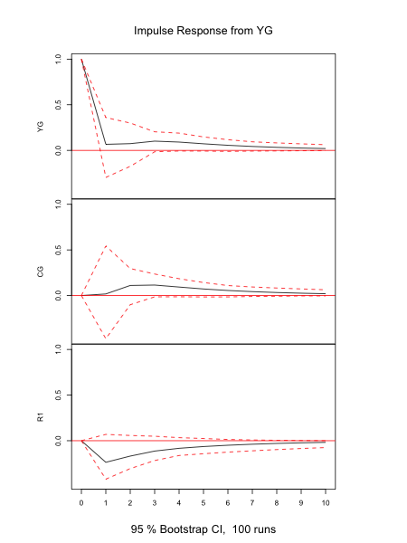
IRF Plots
> # Plot IRFs
> png('irfYG.png',height=8,width=6,units='in',res=150)
> plot(irfEst,names='YG')
> dev.off()
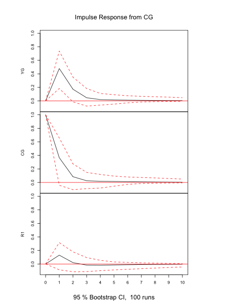
> png('irfCG.png',height=8,width=6,units='in',res=150)
> plot(irfEst,names='CG')
> dev.off()
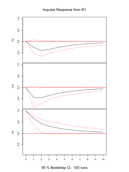
> png('irfR1.png',height=8,width=6,units='in',res=150)
> plot(irfEst,names='R1')
> dev.off()
IRF Plots
IRF Plots
IRF Plots
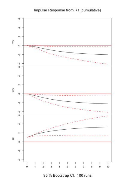
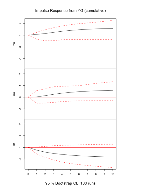
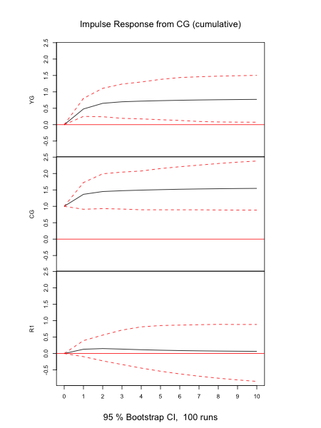
Cumulative IRF Plots
> # Plot cumulative IRFs
> png('irfCumYG.png',height=8,width=6,units='in',res=150)
> plot(irfEstCum,names='YG')
> dev.off()
> png('irfCumCG.png',height=8,width=6,units='in',res=150)
> plot(irfEstCum,names='CG')
> dev.off()
> png('irfCumR1.png',height=8,width=6,units='in',res=150)
> plot(irfEstCum,names='R1')
> dev.off()
Cumulative IRF Plots
Cumulative IRF Plots
Cumulative IRF Plots