Time Series Models of Volatility
Motivation
In many econometric applicaitons, model errors are heteroscedastic.
- In addition to non-constant variance, the variance of the errors may be autocorrelated through time.
- Financial time series have given rise to a rich literature in time series modeling of volatility.
- However, non-financial time series may exhibit time-varying volatility.
Motivation
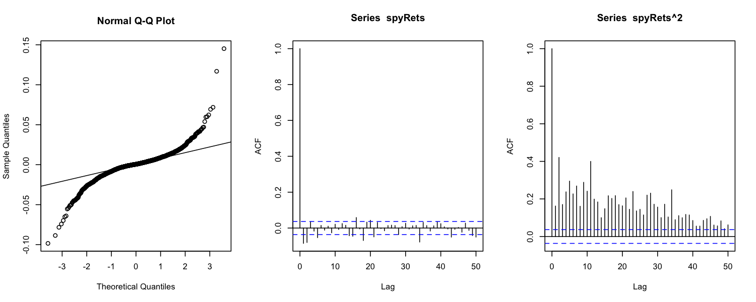
At most time scales, financial returns are known to exhibit:
- Little or no serial correlation.
- Dependence/serial correlation in the second moment.
- Heavy tails, relative to a Gaussian distribution.
Motivation
library(quantmod)
getSymbols('SPY')
spyRets = dailyReturn(Cl(SPY))
png(filename='spyQQACF.png',,height=4,width=10,units='in',res=150)
par(mfrow=c(1,3))
qqnorm(spyRets)
qqline(spyRets)
acf(spyRets,lag.max=50)
acf(spyRets^2,lag.max=50)
dev.off()
Motivation
Basic Model
Consider the following model
- The mean, \(\smash{\mu_t}\), may follow a linear time series process
- The variables \(\smash{\{x_{it}\}}\) are exogenous explanatory variables (e.g. the market return, for the CAPM, or dummy variables for month/week/day effects).
Basic Model
Time series models of volatility augment the model of the mean with a process that governs conditional volatility, \(\smash{\sigma_t}\).
- Some models specify a deterministic process for volatility (\(\smash{ARCH}\)/\(\smash{GARCH}\)).
- Others specify a random process (stochastic volatility).
The \(\smash{ARCH}\) Model
Engle (1982) proposed the following model for volatility
where \(\smash{\alpha_0 > 0}\) and \(\smash{\alpha_i \geq 0}\) for \(\smash{i=1,\ldots,m}\).
- Recall, \(\smash{\varepsilon_t \sim N(0,\sigma_t^2)}\).
- Alternatively, we could write \(\smash{\varepsilon_t = \sigma_t z_t}\), where \(\smash{z_t \sim N(0,1)}\).
\(\smash{ARCH}\) Order
Define \(\smash{\eta_t = \varepsilon_t^2 - \sigma_t^2}\).
- It can be shown that \(\smash{\{\eta_t\}}\) is an uncorrelated, zero-mean series (not necessarily i.i.d.).
- Thus the \(\smash{ARCH}\) model can be written as
- As a result, the order can be diagnosed using the tools of \(\smash{AR}\) order determination (PACF).
- This is done on the residuals, after estimating the mean equation.
Notes on \(\smash{ARCH}\)
- It can be shown that the \(\smash{ARCH}\) model results in excess kurthosis (relative to a Normal).
- The model parameters must be restricted in order to maintain finite unconditional variance and positive conditional variance.
\(\smash{ARCH}\) Estimation
Under the assumption of Normality, the conditional likelihood function is
- MLE is conducted with an interative approach:
- Compute a set of observed residuals \(\smash{\{\varepsilon_t\}}\).
- For a candidate estimate of the parameters, iteratively compute \(\smash{\{\sigma_t^2\}_{m+1}^T}\) with the variance equation and evaluate the likelihood.
- Update the parameters and repeat.
- MLE is often conducted with a \(\smash{t}\) distribution or generalized error distribution.
The \(\smash{GARCH}\) Model
Bollerslev (1986) proposed the following extension to the \(\smash{ARCH}\) model:
where \(\smash{\alpha_0 > 0}\), \(\smash{\alpha_i\geq 0}\), \(\smash{\beta_j\geq 0}\), and \(\smash{\sum_{i=1}^{\max(m,s)} (\alpha_i+\beta_i) < 1}\) for \(\smash{i=1,\ldots,m}\).
Notes on \(\smash{GARCH}\)
- \(\smash{GARCH}\) is often preferred to \(\smash{ARCH}\) because it requires far fewer parameters.
- MLE is conducted in a similar fashion, but requires an initial condition for \(\smash{\{\sigma_t\}_{m-s+1}^m}\).
- As with \(\smash{ARCH}\) models, \(\smash{GARCH}\) models feature excess kurtosis.
- Many refinements of the \(\smash{GARCH}\) model have been developed to account for asymmetry in volatility and other features.
Stochastic Volatility
Stochastic volatility models are an alternative to deterministic models of volatility (\(\smash{ARCH}\)/\(\smash{GARCH}\)).
- Consider the simple model of Taylor (1986):
- \(\smash{u_t}\) may be correlated with the return innovation \(\smash{\varepsilon_t}\).
Stochastic Volatility Estimation
The Kalman filter can be used to estimate the stochastic volatility model above.
- Consider the state-space system of Nelson (1988):
- The Kalman filter cannot be used for other, nonlinear stochastic volatility models.
- Hamilton (1989) developed a nonlinear filtering method, similar to the Kalman filter, for such problems.