Finance Preliminaries
Introduction
Our objective is to learn the theory and application of time series methods.
- We will focus on financial time series applications.
- The methods in this course are broadly applicable to any type of time series.
- We will use the R programming environment to work with financial time series data.
- The quantmod library will be especially useful:
> install.packages("quantmod")
Time Series Example
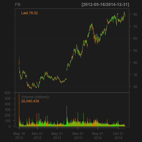
Let’s plot the historical prices for Facebook (FB).
> library(quantmod)
> getSymbols("FB",src="google", from="2012-01-01", to="2014-12-31")
> png(filename="fb.png")
> chartSeries(FB)
> dev.off()
Plot of Facebook Price
Facebook Returns
To plot just the closing prices:
> chartSeries(Cl(FB))
> chartSeries(FB$FB.Close)
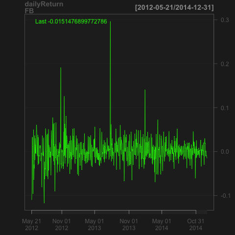
Or daily returns:
> chartSeries(dailyReturn(Cl(FB)))
Plot of Facebook Returns
One-Period Return
Let \(P_t\) be the price of an asset at time \(t\).
- The gross return of the asset between dates \(t-1\) and \(t\) is:
- The net return is:
- Note that the return can be computed between any two dates (i.e. daily, weekly, monthly, etc).
Multi-Period Return
The \(k\) -period gross return between dates \(t-k\) and \(t\) is:
- The \(k\) -period net return is:
Logarithmic Approximation
In general, for any small value \(\smash{\varepsilon > 0}\):
Thus,
Furthermore, by the definition of gross returns,
Approximation for Multiperiod Returns
A similar relationship holds for the \(k\) -period net return:
Time Intervals
The interval of time for returns is of vital importance for understanding the data.
- Daily returns are very different from weekly, monthly, annual, etc. returns.
- Intra-day returns at various time scales (millisecond, second, minute) are very different from each other.
Aggregating Trading Intervals
When aggregating returns, we consider the following.
- There are approximately 250 trading days in a year.
- There are approximately 22 trading days in a month.
- There are 5 trading days in a week.
- U.S. equities markets are open from 9:30 am to 4:00 pm Eastern time - 6.5 hours each day.
- Thus there are approximately 6.5 hours, or 390 minutes or 23,400 seconds or 23,400,000 milliseconds in a trading day.
- Similarly, there are approximately 1625 trading hours, 97,500 trading minutes, 5,850,000 trading seconds and 5,850,000,000 trading milliseconds in a year.
Aggregating Returns
To aggregate net returns, we simply add them:
For example, to annualize daily returns,
Example of Aggregating Returns
Get Exxon Mobile equities data for the week of March 23rd, 2015.
> getSymbols("XOM", from="2015-03-23", to="2015-03-27")
[1] "XOM"
> XOM
           XOM.Open XOM.High XOM.Low XOM.Close XOM.Volume XOM.Adjusted
2015-03-23    85.02    85.78   85.01     85.43   17163200        85.43
2015-03-24    85.30    85.78   84.50     84.52   10099500        84.52
2015-03-25    85.05    85.57   84.77     84.86   11816000        84.86
2015-03-26    85.30    85.57   84.09     84.32   14388500        84.32
2015-03-27    84.04    84.05   83.33     83.58   11094600        83.58
- What are the daily returns?
- What is the weekly return?
Asset Classes
There are several broad classes of assets traded in financial markets.
- Equities.
- Futures.
- Options.
- Bonds.
- Currencies.
Indices
Indices are synthetic portfolios of assets that are not typically traded.
- The S&P 500 index is a portfolio of 500 equities and is not traded.
- To hold the S&P 500 index, one can:
- Purchase the 500 component equities in the correct proportions.
- Purchase shares in a mutual fund that tracks the index.
- Purchase shares of the SPY exchange traded fund (ETF).
- Purchase futures contracts on SPX.
Important Indices
- S&P 500 (SPX).
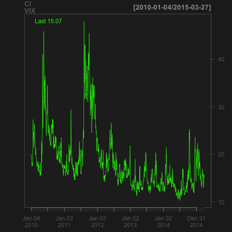
- VIX - portfolio of S&P 500 options which represents the expected value of a one-standard deviation move in the S&P 500 index over the next month (in annual terms).
- On March 30th, 2015, the closing value for VIX was 14.51 and the closing value for SPX 2086.24.
- Hence, the market expects the standard deviation of the SPX to be \(14.51/\sqrt{12} = 4.19\) percent or \(\smash{0.0419\times 2086.24 = 87.39}\) index points.
Important Assets
- SPY - SPX ETF.
- E-mini - Futures contract on the SPX.
- SPX Options.
- SPY Options.
- VIX Options.
- VIX Futures.
Near-Month VX Futures
> install.packages("Quandl")
> library(Quandl)
> VX1 = Quandl("OFDP/FUTURE_VX1",type="xts")
> chartSeries(VX1)

E-mini Near-Month Returns
> ES1 = Quandl("OFDP/FUTURE_ES1",start_date="2007-01-01",end_date="2015-03-27",type="xts")
> chartSeries(dailyReturn(ES1$Open))
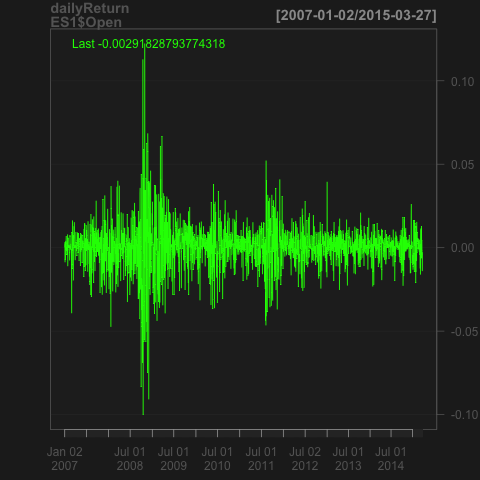
Important Features of Returns
What do you notice about the E-mini returns?