Moving Average Processes
White Noise Revisited
White noise, \(\smash{\{\varepsilon_t\}_{t=-\infty}^{\infty}}\), is a fundamental building block of canonical time series processes.
- We will often use the abbreviation \(\smash{\{\varepsilon_t\}}\).
\(\smash{MA(1)}\)
Given white noise \(\smash{\{\varepsilon_t\}}\), consider the process
where \(\smash{\mu}\) and \(\smash{\theta}\) are constants.
- This is a first-order moving average or \(\smash{MA(1)}\) process.
- We can rewrite in terms of the lag operator:
where \(\smash{\theta(L) = (1+\theta L)}\).
\(\smash{MA(1)}\) Mean and Variance
The mean of the first-order moving average process is
\(\smash{MA(1)}\) Autocovariances
\(\smash{MA(1)}\) Autocovariances
- If \(\smash{j = 0}\)
- If \(\smash{j = 1}\)
- If \(\smash{j > 1}\), all of the expectations are zero: \(\smash{\gamma_j = 0}\).
\(\smash{MA(1)}\) Stationarity and Ergodicity
Since the mean and autocovariances are independent of time, an \(\smash{MA(1)}\) is weakly stationary.
- This is true for all values of \(\smash{\theta}\).
The condition for ergodicity of the mean also holds:
- If \(\smash{\{\varepsilon_t\}}\) is Gaussian then \(\smash{\{Y_t\}}\) is also ergodic for all moments.
\(\smash{MA(1)}\) Autocorrelations
The autocorrelations of an \(\smash{MA(1)}\) are
- \(\smash{j = 0}\): \(\smash{\rho_0 = 1}\) (always).
- \(\smash{j = 1}\):
- \(\smash{j > 1}\): \(\smash{\rho_j = 0}\).
- If \(\smash{\theta > 0}\), first-order lags of \(\smash{Y_t}\) are positively autocorrelated.
- If \(\smash{\theta < 0}\), first-order lags of \(\smash{Y_t}\) are negatively autocorrelated.
- \(\smash{\max\{\rho_1\} = 0.5}\) and occurs when \(\smash{\theta = 1}\).
- \(\smash{\min\{\rho_1\} = -0.5}\) and occurs when \(\smash{\theta = -1}\).
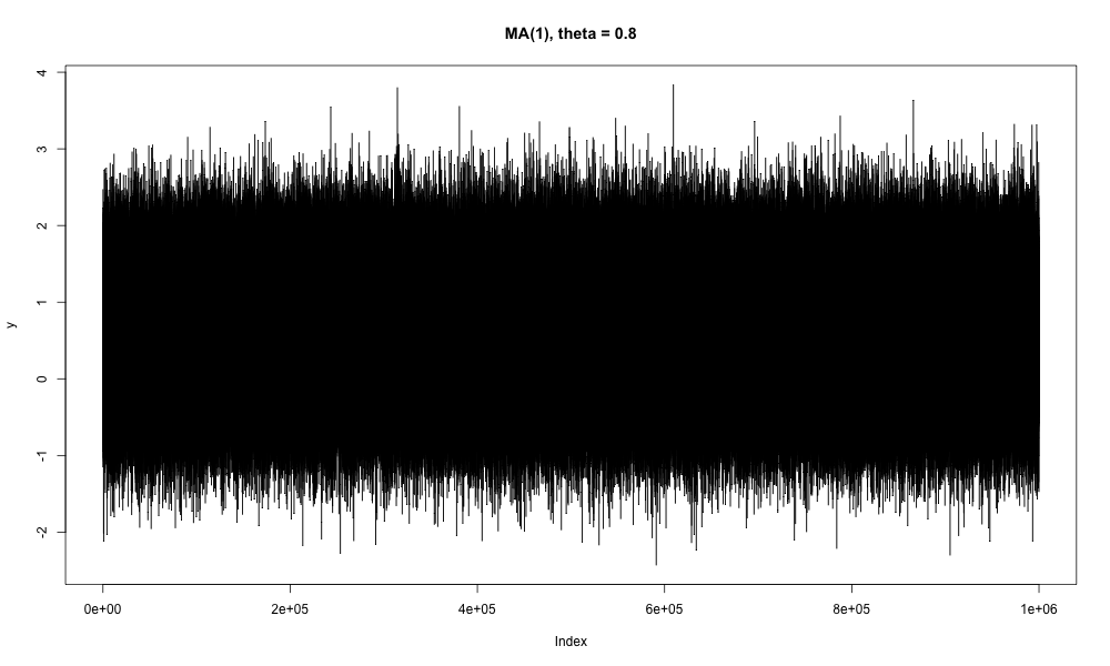
\(\smash{MA(1)}\) Example
#################################################################
# Simulate MA(1)
#################################################################

# Simulate MA(1)
N = 1000000;
sigma = 0.5;
eps = rnorm(N, 0, sigma);

# Simulate
mu = 0.61;
theta = 0.8;
y = mu + eps[2:N] + theta*eps[1:(N-1)];

# Plot
png(file="ma1ExampleSeries.png", height=800, width=1000)
plot(y, main=paste("MA(1), ",expression(theta)," = ",theta, sep=""),type="l")
dev.off()
\(\smash{MA(1)}\) Example
\(\smash{MA(1)}\) Autocorrelations
#################################################################
# Plot ACF for MA(1)
#################################################################

# Plot the empirical acf
png(file="ma1ACF.png", height=800, width=1000)
acf(y, main="Autocorrelations for MA(1)")
dev.off()
\(\smash{MA(1)}\) Autocorrelations
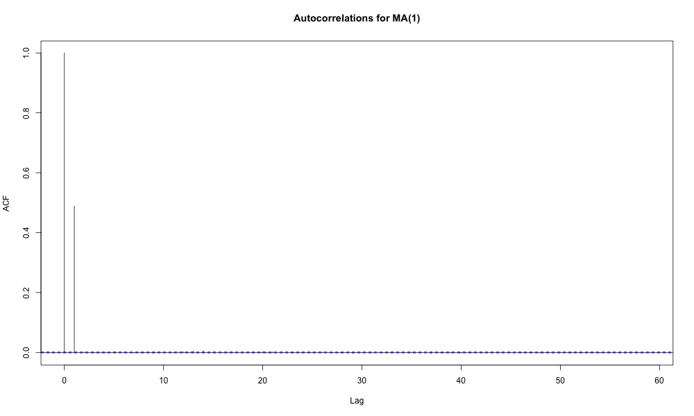
\(\smash{MA(1)}\) Autocorrelations
#################################################################
# Plot lag 1 autocorrelation for different MA(1)
#################################################################

# Construct a grid of first-order coefficients
N = 10000;
thetaGrid = seq(-3, 3, length=N);

# Compute the lag 1 autocorrelations
rho1 = thetaGrid/(1+thetaGrid^2);

# Plot
png(file="ma1Lag1.png", height=600, width=1000)
plot(thetaGrid, rho1, type='l', xlab=expression(theta), ylab=expression(rho[1]),
     main="Lag 1 Autocorrelation for MA(1)")
abline(h=0);
abline(h=0.5, lty=3);
abline(h=-0.5, lty=3);
dev.off()
\(\smash{MA(1)}\) Autocorrelations
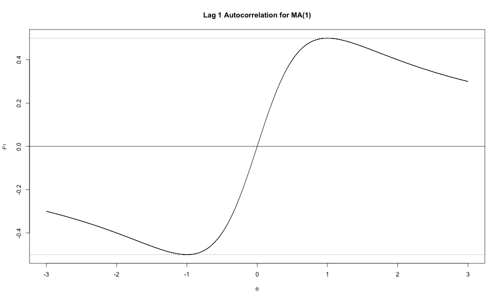
\(\smash{MA(1)}\) Autocorrelations
From the figure above we see that there are two values of \(\smash{\theta}\) that generate each value of
\(\smash{\rho_1}\).
- In fact, \(\smash{\theta}\) and \(\smash{1/\theta}\) correspond to the same \(\smash{\rho_1}\):
\(\smash{MA(1)}\) Autocorrelations
Consider:
Then:
\(\smash{MA(q)}\)
A \(\smash{q}\) th-order moving average or \(\smash{MA(q)}\) process is
where \(\smash{\mu, \theta_1, \ldots, \theta_q}\) are any real numbers.
- We can rewrite in terms of the lag operator:
where \(\smash{\theta(L) = (1+\theta_1 L^1 + \ldots + \theta_q L^q)}\).
\(\smash{MA(q)}\) Mean
As with the \(\smash{MA(1)}\):
\(\smash{MA(q)}\) Autocovariances
- For \(\smash{j > q}\), all of the products result in zero expectations: \(\smash{\gamma_j = 0}\), for \(\smash{j > q}\).
For \(\smash{j = 0}\), the squared terms result in nonzero expectations, while the cross products lead to zero expectations:
\[\smash{\gamma_0 = \text{E}[\varepsilon^2_t ] + \theta^2_1 \text{E}[\varepsilon^2_{t-1}] + \ldots + \theta^2_q \text{E}[\varepsilon^2_{t-q}] = \left(1 + \sum_{j=1}^q \theta^2_j\right) \sigma^2.}\]
\(\smash{MA(q)}\) Autocovariances
- For \(\smash{j = \{1,2,\ldots,q\}}\), the nonzero expectation terms are
The autocovariances can be stated concisely as
where \(\smash{\theta_0 = 1}\).
\(\smash{MA(q)}\) Autocorrelations
The autocorrelations can be stated concisely as
where \(\smash{\theta_0 = 1}\).
\(\smash{MA(2)}\) Example
For an \(\smash{MA(2)}\) process
\(\smash{MA(q)}\) Stationarity and Ergodicity
Since the mean and autocovariances are independent of time, an \(\smash{MA(q)}\) is weakly stationary.
- This is true for all values of \(\smash{\{\theta_j\}_{j=1}^q}\).
The condition for ergodicity of the mean also holds:
- If \(\smash{\{\varepsilon_t\}}\) is Gaussian then \(\smash{\{Y_t\}}\) is also ergodic for all moments.
\(\smash{MA(\infty)}\)
If \(\smash{\theta_0 = 1}\), the \(\smash{MA(q)}\) process can be written as
- If we take the limit \(\smash{q \to \infty}\):
where \(\smash{\theta(L) = \sum_{j=0}^{\infty} \theta_j L^j}\).
- It can be shown that an \(\smash{MA(\infty)}\) process is weakly stationary if
\(\smash{MA(\infty)}\)
Since absolute summability implies square summability
an \(\smash{MA(\infty)}\) process satisfying absolute summability is also weakly stationary.
- In general
\(\smash{MA(\infty)}\) Moments
Following the same reasoning as above,
- \(\smash{\sum_{j=0}^{\infty} |\theta_j| \Rightarrow \sum_{j=0}^{\infty} |\gamma_j|}\).
- So if the \(\smash{MA(\infty)}\) has absolutely summable coefficients, it is ergodic for the mean.
- Further, if \(\smash{\{\varepsilon_t\}}\) is Gaussian then \(\smash{\{Y_t\}}\) is also ergodic for all moments.