Autoregressive Processes¶

\(\smash{AR(1)}\) Process¶

Given white noise \(\smash{\{\varepsilon_t\}}\), consider the process

\[\smash{Y_t = c + \phi Y_{t-1} + \varepsilon_t,}\]

where \(\smash{c}\) and \(\smash{\phi}\) are constants.

This is a first-order autoregressive or \(\smash{AR(1)}\) process.

We can rewrite in terms of the lag operator:

\[\smash{(1-\phi L) Y_t = c + \varepsilon_t.}\]

\(\smash{AR(1)}\) as \(\smash{MA(\infty)}\)¶

From our discussion of lag operators, we know that if \(\smash{|\phi| < 1}\)

\[\begin{split}\begin{align*} Y_t & = (1-\phi L)^{-1} c + (1-\phi L)^{-1} \varepsilon_t \\ & = \left(\sum_{i=0}^{\infty} \phi^i L^i\right) c + \left(\sum_{i=0}^{\infty} \phi^i L^i\right) \varepsilon_t \\ & = \left(\sum_{i=0}^{\infty} \phi^i\right) c + \left(\sum_{i=0}^{\infty} \phi^i L^i\right) \varepsilon_t \\ & = \frac{c}{1-\phi} + \theta(L) \varepsilon_t, \end{align*}\end{split}\]

where

\[\smash{\theta(L) = \sum_{i=0}^{\infty} \theta_i L^i = \sum_{i=0}^{\infty} \phi^i L^i = \phi(L)^{-1}.}\]

\(\smash{AR(1)}\) as \(\smash{MA(\infty)}\)¶

Restating, when \(\smash{|\phi| < 1}\)

\[\smash{Y_t = \frac{c}{1-\phi} + \theta(L) \varepsilon_t = \frac{c}{1-\phi} + \sum_{i=0}^{\infty} \phi^i \varepsilon_{t-i}.}\]

This is an \(\smash{MA(\infty)}\) with \(\smash{\mu = c/(1-\phi)}\) and \(\smash{\theta_i = \phi^i}\).

Note that \(\smash{|\phi| < 1}\) implies

\[\smash{\sum_{j=0}^{\infty} |\theta_j| = \sum_{j=0}^{\infty} |\phi|^j < \infty,}\]

which means that \(\smash{Y_t}\) is weakly stationary.

Expectation of \(\smash{AR(1)}\)¶

Assume \(\smash{Y_t}\) is weakly stationary: \(\smash{|\phi| < 1}\).

\[\begin{split}\begin{align*} \text{E}[Y_t] & = c + \phi \text{E}[Y_{t-1}] + \text{E}[\varepsilon_t] \\ & = c + \phi \text{E}[Y_t] \\ \Rightarrow \text{E}[Y_t] & = \frac{c}{1-\phi}. \end{align*}\end{split}\]

A Useful Property¶

If \(\smash{Y_t}\) is weakly stationary,

\[\smash{Y_{t-j} - \mu = \sum_{i=0}^{\infty} \phi^i \varepsilon_{t-j-i}.}\]

That is, for \(\smash{j \geq 1}\), \(\smash{Y_{t-j}}\) is a function of lagged values of \(\smash{\varepsilon_t}\) and not \(\smash{\varepsilon_t}\) itself.

As a result, for \(\smash{j \geq 1}\)

\[\begin{align*} \text{E}\left[(Y_{t-j}-\mu) \varepsilon_t\right] & = \sum_{i=0}^{\infty} \phi^i \text{E}[\varepsilon_t \varepsilon_{t-j-i}] = 0. \end{align*}\]

Variance of \(\smash{AR(1)}\)¶

Given that \(\smash{\mu = c/(1-\phi)}\) for weakly stationary \(\smash{Y_t}\):

\[\begin{split}\begin{gather*} Y_t = \mu(1-\phi) + \phi Y_{t-1} + \varepsilon_t \\ \Rightarrow (Y_t - \mu) = \phi(Y_{t-1} - \mu) + \varepsilon_t. \end{gather*}\end{split}\]

Squaring both sides and taking expectations:

\[ \begin{align}\begin{aligned}\begin{split}\begin{align*} \text{E}\left[(Y_t-\mu)^2\right] & = \phi^2 \text{E}\left[(Y_{t-1}-\mu)^2\right] + 2\phi \text{E}\left[(Y_{t-1}-\mu)\varepsilon_t\right] + \text{E}[\varepsilon_t^2] \\ & = \phi^2 \text{E}\left[(Y_t-\mu)^2\right] + \sigma^2 \end{align*}\end{split}\\\begin{split}\begin{gather*} \Rightarrow (1-\phi^2) \gamma_0 = \sigma^2 \\ \Rightarrow \gamma_0 = \frac{\sigma^2}{1-\phi^2} \end{gather*}\end{split}\end{aligned}\end{align} \]

Autocovariances of \(\smash{AR(1)}\)¶

For \(\smash{j \geq 1}\),

\[\begin{split}\begin{align*} \gamma_j & = \text{E}\left[(Y_t-\mu)(Y_{t-j}-\mu)\right] \\ & = \phi \text{E}[(Y_{t-1}-\mu)(Y_{t-j} - \mu)] + \text{E}[\varepsilon_t (Y_{t-j} - \mu)] \\ & = \phi \gamma_{j-1} \\ & \vdots \\ & = \phi^j \gamma_0. \end{align*}\end{split}\]

Autocorrelations of \(\smash{AR(1)}\)¶

The autocorrelations of an \(\smash{AR(1)}\) are

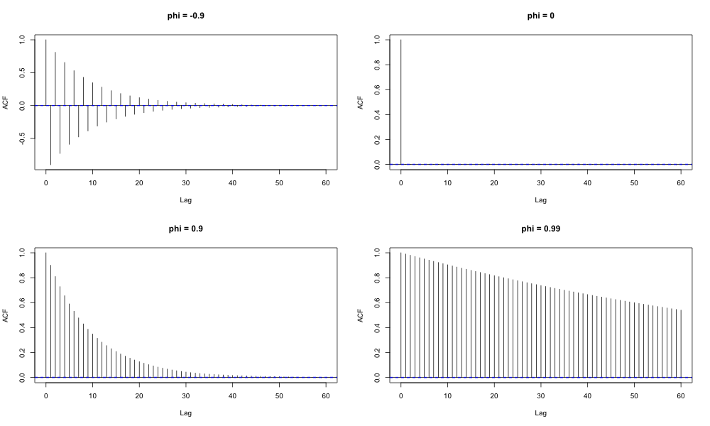
\[\smash{\rho_j = \frac{\gamma_j}{\gamma_0} = \phi^j, \,\,\,\, \forall j \geq 0.}\]

Since we assumed \(\smash{|\phi| < 1 }\), the autocorrelations decay exponentially as \(\smash{j}\) increases.

Note that if \(\smash{\phi \in (-1,0)}\), the autocorrelations decay in an oscillatory fashion.

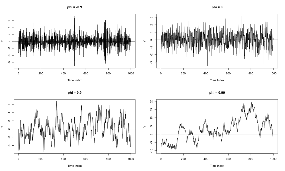
Examples of \(\smash{AR(1)}\) Processes¶

###########################################################
# Simulate AR(1) processes for different values of phi
###########################################################

# Number of simulated points
nSim = 1000000;

# Values of phi to consider
phi = c(-0.9, 0, 0.9, 0.99);

# Draw one set of shocks and use for each AR(1)
eps = rnorm(nSim, 0, 1);

# Matrix which stores each AR(1) in columns
y = matrix(0, nrow=nSim, ncol=length(phi));

# Each process is intialized at first shock
y[1,] = eps[1];

# Loop over each value of phi
for(j in 1:length(phi)){

    # Loop through the series, simulating the AR(1) values
    for(i in 2:nSim){
        y[i,j] = phi[j]*y[i-1,j]+eps[i]
    }
 }

Examples of \(\smash{AR(1)}\) Processes¶

###########################################################
# Plot the AR(1) realizations for each phi
###########################################################

# Only plot a subset of the whole simulation
plotInd = 1:1000

# Specify a plot grid
png(file="ar1ExampleSeries.png", height=600, width=1000)
par(mfrow=c(2,2))

# Loop over each value of phi
for(j in 1:length(phi)){
    plot(plotInd,y[plotInd,j], type='l', xlab='Time Index',
         ylab="Y", main=paste(expression(phi), " = ", phi[j], sep=""))
    abline(h=0)
 }
 graphics.off()

Examples of \(\smash{AR(1)}\) Processes¶

\(\smash{AR(1)}\) Autocorrelations¶

###########################################################
# Plot the sample ACFs for each AR(1) simulation
# For large nSim, sample ACFs are close to true ACFs
###########################################################

# Specify a plot grid
png(file="ar1ExampleACF.png", height=600, width=1000)
par(mfrow=c(2,2))

# Loop over each value of phi
for(j in 1:length(phi)){
    acf(y[,j], main=paste(expression(phi), " = ", phi[j], sep=""))
}
graphics.off()

\(\smash{AR(1)}\) Autocorrelations¶

\(\smash{AR(p)}\) Process¶

Given white noise \(\smash{\{\varepsilon_t\}}\), consider the process

\[\smash{Y_t = c + \phi_1 Y_{t-1} + \phi_2 Y_{t-2} + \ldots + \phi_p Y_{t-p} + \varepsilon_t,}\]

where \(\smash{c}\) and \(\smash{\{\phi\}_{i=1}^p}\) are constants.

This is a \(\smash{p}\) th-order autoregressive or \(\smash{AR(p)}\) process.

We can rewrite in terms of the lag operator:

\[\smash{\phi(L) Y_t = c + \varepsilon_t.}\]

where

\[\smash{\phi(L) = (1-\phi_1 L - \phi_2 L^2 - \ldots - \phi_p L^p).}\]

\(\smash{AR(p)}\) as \(\smash{MA(\infty)}\)¶

From our discussion of lag operators,

\[\smash{Y_t = \phi(L)^{-1} c + \phi(L)^{-1} \varepsilon_t,}\]

if the roots of \(\smash{\phi(L)}\) all lie outside the unit circle.

In this case, \(\smash{\phi(L) = (1-\lambda_1 L)(1-\lambda_2 L) \cdots (1-\lambda_pL).}\)

If the roots, \(\smash{\frac{1}{|\lambda_i|} > 1}\), \(\smash{\forall i}\) then \(\smash{|\lambda_i| < 1}\),

\(\smash{\forall i}\) and

\[\begin{split}\begin{align*} \phi(L)^{-1} & = (1-\lambda_1 L)^{-1}(1-\lambda_2 L)^{-1} \cdots (1-\lambda_pL)^{-1} \\ & = \left(\sum_{j=0}^{\infty} \lambda_1^j L^j\right) \left(\sum_{j=0}^{\infty} \lambda_2^j L^j\right) \cdots \left(\sum_{j=0}^{\infty} \lambda_p^j L^j\right). \end{align*}\end{split}\]

\(\smash{AR(p)}\) as \(\smash{MA(\infty)}\)¶

For \(\smash{|\lambda_i| < 1}\), \(\smash{\forall i}\)

\(\smash{Y_t}\) is an \(\smash{MA(\infty)}\) with \(\smash{\mu = \phi(L)^{-1} c}\) and \(\smash{\theta(L) = \phi(L)^{-1}}\).

It can be shown that \(\smash{\sum_{i=1}^{\infty} |\theta_i| < \infty}\).

As a result, \(\smash{Y_t}\) is weakly stationary.

Vector Autoregressive Process¶

We can rewrite the \(\smash{AR(p)}\) as

\[\smash{{\bf Y}_t = {\bf c} + \Phi {\bf Y}_{t-1} + {\bf \varepsilon}_t,}\]

where

\[\begin{split}\begin{equation*} {\bf Y}_t = \left[\begin{array}{c} Y_t \\ Y_{t-1} \\ Y_{t-2} \\ \vdots \\ Y_{t-p+1} \end{array} \right] \,\,\,\, \Phi = \left[\begin{array}{ccccc} \phi_1 & \phi_2 & \ldots & \phi_{p-1} & \phi_p \\ 1 & 0 & \ldots & 0 & 0 \\ 0 & 1 & \ldots & 0 & 0 \\ \vdots & \vdots & \ddots & \vdots & \vdots \\ 0 & 0 & \ldots & 1 & 0 \end{array} \right] \,\,\,\,\, {\bf \varepsilon}_t = \left[\begin{array}{c} \varepsilon_t \\ 0 \\ 0 \\ \vdots \\ 0 \end{array} \right], \end{equation*}\end{split}\]

and \(\smash{{\bf c} = (c,c,\ldots,c)'_{1 \times p}}\).

Vector Autoregressive Process¶

It turns out that the values \(\smash{\{\lambda_i\}_{i=1}^p}\) are the \(\smash{p}\) eigenvalues of \(\smash{\Phi}\).

So the eigenvalues of \(\smash{\Phi}\) are the inverses of the roots of the lag polynomial \(\smash{\phi(L)}\).

Hence, \(\smash{\phi(L)^{-1}}\) exists if all \(\smash{p}\) roots of \(\smash{\phi(L)}\) lie outside the unit circle or all \(\smash{p}\) eigenvalues of \(\smash{\Phi}\) lie inside the unit circle.

These conditions ensure weak stationarity of the \(\smash{AR(p)}\) process.

Expectation of \(\smash{AR(p)}\)¶

Assume \(\smash{Y_t}\) is weakly stationary: the roots of \(\smash{\phi(L)}\) lie outside the unit circle.

\[\begin{split}\begin{align*} \text{E}[Y_t] & = c + \phi_1 \text{E}[Y_{t-1}] + \ldots + \phi_p \text{E}[Y_{t-p}] + \text{E}[\varepsilon_t] \\ & = c + \phi_1 \text{E}[Y_t] + \ldots + \phi_p \text{E}[Y_t] \\ \Rightarrow \text{E}[Y_t] & = \frac{c}{1-\phi_1 - \ldots - \phi_p} = \mu. \end{align*}\end{split}\]

Autocovariances of \(\smash{AR(p)}\)¶

Given that \(\smash{\mu = c/(1-\phi_1 - \ldots - \phi_p)}\) for weakly stationary \(\smash{Y_t}\):

\[\begin{split}\begin{gather*} Y_t = \mu(1-\phi_1 - \ldots - \phi_p) + \phi_1 Y_{t-1} + \ldots + \phi_p Y_{t-p} + \varepsilon_t \\ \Rightarrow (Y_t - \mu) = \phi_1(Y_{t-1} - \mu) + \ldots + \phi_p(Y_{t-p} - \mu) + \varepsilon_t. \end{gather*}\end{split}\]

Thus,

\[\begin{split}\begin{align} \gamma_j & = \text{E}\left[(Y_t - \mu) (Y_{t-j} - \mu)\right] \nonumber \\ & = \phi_1 \text{E}\left[(Y_{t-1} - \mu) (Y_{t-j} - \mu)\right] + \ldots \nonumber \\ & \hspace{0.75in} + \phi_p \text{E}\left[(Y_{t-p} - \mu) (Y_{t-j} - \mu)\right] + \text{E}\left[\varepsilon_t (Y_{t-j} - \mu)\right] \nonumber \\ & = \begin{cases} \phi_1 \gamma_{j-1} + \ldots + \phi_p \gamma_{j-p} & \text{ for } j = 1, \ldots \\ \phi_1 \gamma_1 + \ldots + \phi_p \gamma_p + \sigma^2 & \text{ for } j = 0. \end{cases} \label{gammas} \end{align}\end{split}\]

Autocovariances of \(\smash{AR(p)}\)¶

For \(\smash{j = 0, 1, \ldots, p}\), the equations above are a system of \(\smash{p+1}\) equations with \(\smash{p+1}\) unknowns: \(\smash{\{\gamma_j\}_{j=0}^p}\).

\(\smash{\{\gamma_j\}_{j=0}^p}\) can be solved for as functions of \(\smash{\{\phi_j\}_{j=1}^p}\) and \(\smash{\sigma^2}\).

It can be shown that \(\smash{\{\gamma_j\}_{j=0}^p}\) are the first \(\smash{p}\) elements of the first column of \(\smash{\sigma^2 [I_{p^2} - \Phi \otimes \Phi]^{-1}}\), where

\(\smash{\otimes}\) denotes the Kronecker product.

\(\smash{\{\gamma_j\}_{j=p+1}^{\infty}}\) can then be determined using prior values of \(\smash{\gamma_j}\) and \(\smash{\{\phi_j\}_{j=1}^p}\).

Autocorrelations of \(\smash{AR(p)}\)¶

Dividing the autocovariances by \(\smash{\gamma_0}\),

\[\smash{\rho_j = \phi_1 \rho_{j-1} + \ldots + \phi_p \rho_{j-p} \,\,\,\,\,\, \text{ for } j = 1, \ldots}\]