Data Transformations¶

Transformations¶

Data often deviate from normality and exhibit characteristics (skewness, kurtosis) that are difficult to model.

Transforming data using some functional form will often result in observations that are easier to model.

The most typical transformations are the natural logarithm and the square root.

Logarithmic Transformation¶

Given independent and dependent variables, \((x_t, y_t)\), the natural logarithm transformation is appropriate under several circumstances:

\(y_t\) is strictly positive (the log of a negative number does not exist).

\(y_t\) increases exponentially (faster than linearly) as \(x_t\) increases.

The variance in \(y_t\) appears to depend on its mean (heteroskedasticity).

Logarithmic Transformation¶

Consider the relationship

\[y_t = \exp(\beta x_t)\exp(\epsilon_t),\]

where \(\epsilon_t \sim \mathcal{N}(0,\sigma)\).

If \(\epsilon_t \sim \mathcal{N}(0,\sigma)\), then \(\exp(\epsilon_t) \sim \mathcal{LN}(0,\sigma)\).

In this case,

\[\begin{split}E\left[\exp(\epsilon_t)\right] = \exp(0.5\sigma^2) \\\end{split}\]

\[Var\left(\exp(\epsilon_t)\right) = \left(\exp(\sigma^2)-1\right) \exp(\sigma^2).\]

Logarithmic Transformation¶

Thus,

\[\begin{split}E[y_t] = \exp(\beta x_t) \exp(0.5 \sigma^2) \\\end{split}\]

\[Var(y_t) = \exp(2\beta x_t) \left(\exp(\sigma^2)-1\right) \exp(\sigma^2).\]

That is, \(E[y_t]\) grows exponentially with \(x_t\) and \(Var(y_t)\) is heteroskedastic.

Logarithmic Transformation¶

Taking the natural logarithm

\[\log(y_t) = \beta x_t + \epsilon_t,\]

\(E\left[\log(y_t)\right]\) grows linearly with \(x_t\).

\(Var\left(\log(y_t)\right)\) is homoskedastic.

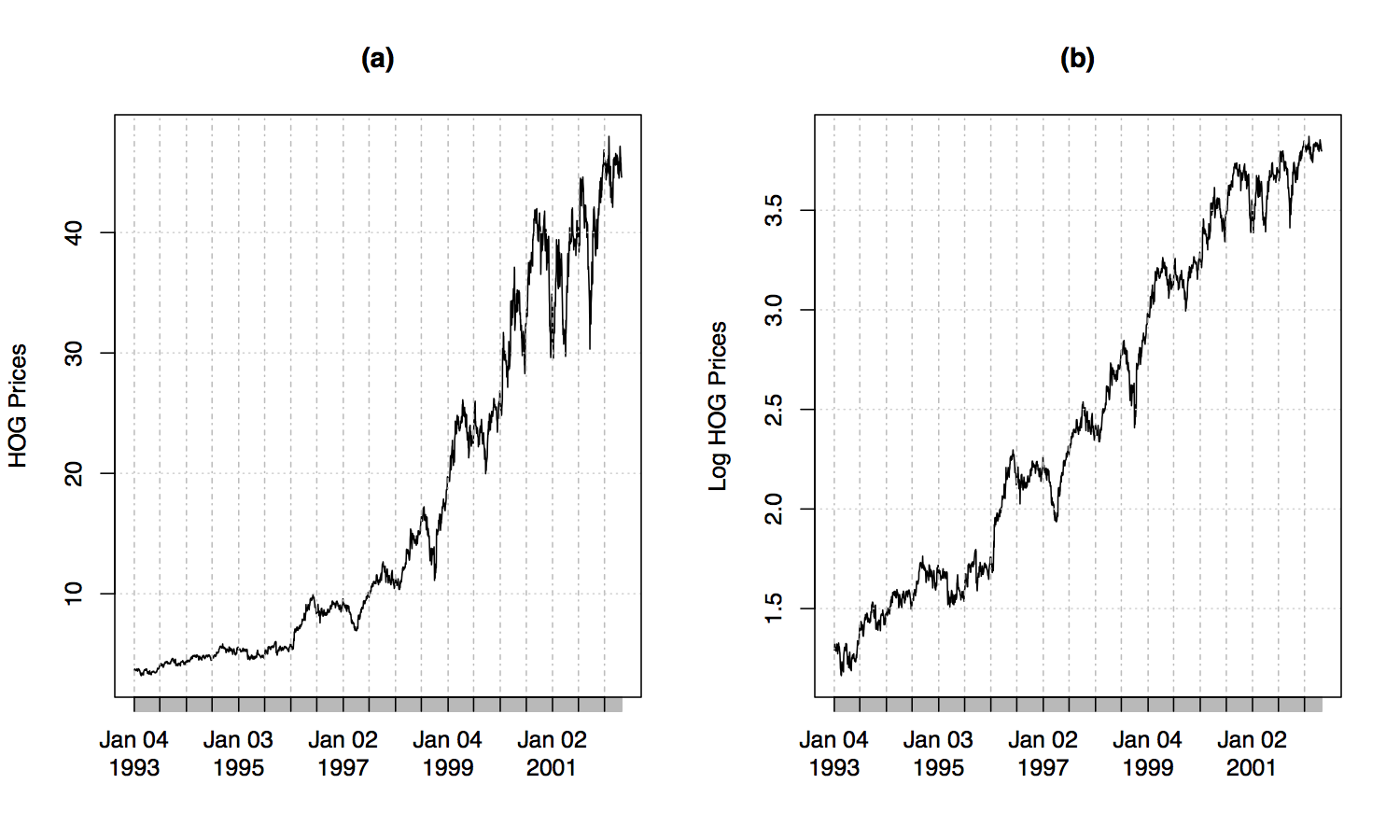
Logarithmic Transformation Example¶

Given, \(\beta = 0.5\) and \(\epsilon_t \sim \mathcal{N}(0,0.15)\), the plot below depicts

\[\begin{split}y_t & = \exp(\beta x_t)\exp(\epsilon_t) \\ \log(y_t) & = \beta x_t + \epsilon_t.\end{split}\]\[.. ifslides::\]\[.. image:: /_static/Transform/logTransExample.png :width: 7.5in :align: center\]

Logarithmic Transformation Example¶

Asset prices often display the characteristics that are suitable for a logarithmic transformation.

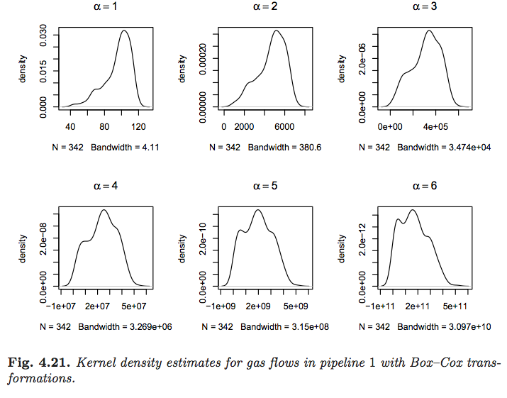
Box-Cox Power Transformations¶

Generally speaking, the set of transformations

\[\begin{split}y^{\alpha} = \begin{cases} \frac{y^{\alpha}-1}{\alpha} & \alpha \neq 0 \\ \log(y) & \alpha = 0, \end{cases}\end{split}\]

Is known as the family of Box-Cox power transformations.

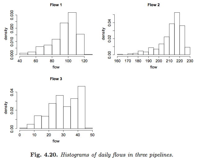
Correcting Skewness and Heteroskedasticity¶

Suppose a set of data observations, \(y_t\), appear to be right skewed and have variance increasing with it’s mean.

A concave transformation with \(\alpha < 1\) will reduce the skewness and stabilize the variance.

The smaller the value of \(\alpha\), the greater the effect of the transformation.

Selecting \(\alpha < 1\) too small may result in left skewness or variance decreasing with the mean (or both).

The \(\alpha\) that creates the most symmetric data may not be the best for stabilizing variance - there may be a tradeoff.

Box Cox Example¶

This plot was taken directly from Ruppert (2011).

Box Cox Example¶

This plot was taken directly from Ruppert (2011).

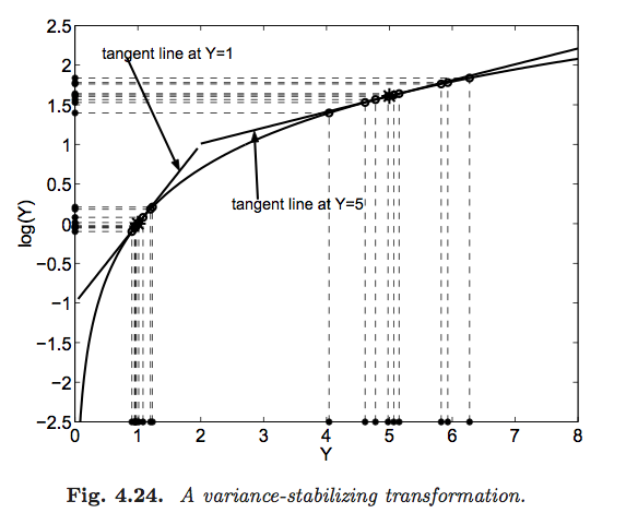
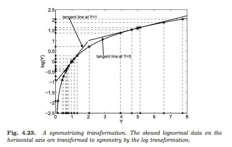
Geometry of Transformations¶

Transformations can be beneficial because they stretch observations apart in some regions and push them together in other regions.

If data are right skewed, then a concave transformation will
- Stretch the distances between observations at the lower end of the distribution.
- Compress the distances between observations at the upper end of the distribution.

The degree of stretching and compressing will depend on the derivatives of the transformation function.

Geometry of Transformations¶

For two values, \(x\) and \(x'\) close to each other, Taylor’s theorem says

\[\begin{split}|h(x) - h(x')| & \approx h'(x) |x-x'|.\end{split}\]

\(h(x)\) and \(h(x')\) will be pushed apart where \(h'(x)\) is large.

\(h(x)\) and \(h(x')\) will be pushed together where \(h'(x)\) is small.

\(h'(x)\) is a decreasing function of \(x\) if \(h\) is concave.

Geometry of Transformations¶

This plot was taken directly from Ruppert (2011).

Geometry of Transformations¶

Similarly, if the variance of a data set increases with its mean, a concave transformation will

Push more variable values closer together (for large values of the data).

Push less variable values further apart (for small values of the data).

Geometry of Transformations¶

This plot was taken directly from Ruppert (2011).