Resampling¶

Properties of Estimators¶

We’ve now seen that estimation is not enough.

We often want to know about properties of estimators.

For example, what is the standard error of an estimator?

Remember that before data is observed, an estimator is a random variable itself.

As an example, \(\bar{Y}\) is a sum of random variables divided by a constant value.

Before \(\{Y_i\}_{i=1}^n\) is observed, \(\bar{Y}\) is random and has its own variance and standard deviation.

Resampling¶

It is often challenging or impossible to compute certain characteristics of estimators.

We would like to replace theoretical calculations with Monte Carlo simulation, which draws additional samples from the population.

Sampling from the true population is typically impossible.

Resampling¶

We substitute sampling from the true population with sampling from the observed sample.

This is referred to as resampling.

If the sample is a good representation of the true population, then sampling from the sample should approximate sampling from the population.

Bootstrapping¶

Suppose the original sample has \(n\) data observations.

Bootstrapping involves drawing \(B\) new samples of size \(n\) from the original sample.

Each bootstrap sample is done with replacement.

Otherwise, the bootstrap samples would all be identical to the original sample (why?).

Drawing with replacement allows each bootstrap observation to be drawn in an \(i.i.d.\) fashion from the sample.

So, the original sample plays the role of the population.

Bootstrap Estimates¶

Let \(\theta\) be a parameter of interest and let \(\hat{\theta}\) denote an estimate of \(\theta\) using a sample of data, \(\{y_i\}_{i=1}^n\).

\(\hat{\theta}\) might be calculated by maximum likelihood estimation.

We could create \(B\) new samples from \(\{y_i\}_{i=1}^n\) by resampling with replacement.

For each new sample \(j = 1, \ldots, B\), we could compute \(\hat{\theta}^*_j\) in the exact way \(\hat{\theta}\) was computed with \(\{y_i\}_{i=1}^n\).

Bootstrap Estimates¶

One way to estimate \(E[\hat{\theta}]\) is by averaging the bootstrap estimates:

\[E[\hat{\theta}] \approx \bar{\hat{\theta}}^* = \frac{1}{B} \sum_{j=1}^B \hat{\theta}^*_j.\]

Estimating Bias¶

True bias for an estimator is defined as

\[\text{BIAS}(\hat{\theta}) = E[\hat{\theta}] - \theta.\]

We can approximate the population average, \(E[\hat{\theta}]\), with a bootstrap average, \(\bar{\hat{\theta}}^*\):

\[\text{BIAS}_{\text{boot}}(\hat{\theta}) = \bar{\hat{\theta}}^* - \hat{\theta}.\]

We replaced the true population value, \(\theta\), with the sample value, \(\hat{\theta}\), since the sample substitutes for the population.

Estimating Standard Error¶

The true standard deviation of \(\hat{\theta}\) can be estimated with the bootstrap estimates:

\[s_{\text{boot}}(\hat{\theta}) = \sqrt{\frac{1}{B-1} \sum_{j=1}^B \left(\hat{\theta}^*_j - \bar{\hat{\theta}}^* \right)^2}.\]

Example: Pareto Distribution¶

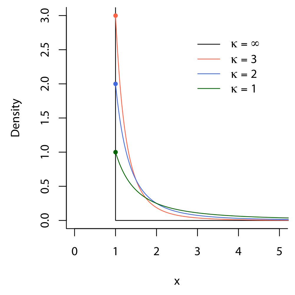
Suppose we have a sample of random variables drawn from a Pareto distribution:

\[Y_i \stackrel{i.i.d.}{\sim} \mathcal{P}(\alpha, \beta), \qquad i=1,\ldots, n.\]

The density of each \(Y_i\) is

\[f(y|\alpha, \beta) = \frac{\beta \alpha^\beta}{y^{\beta+1}}.\]

If \(Y_i \sim \mathcal{P}(\alpha, \beta)\), then \(\alpha > 0\), \(\beta > 0\) and \(Y_i > \alpha\).

\(\alpha\) is a parameter dictating the minimum possible value of \(Y_i\) and \(\beta\) is a shape parameter.

Example: Pareto Distribution¶

In the graph below, \(\beta = \kappa\).

Example: Pareto Distribution¶

The joint density of \({\bf Y} = (Y_1, \ldots, Y_n)'\) is

\[f_{{\bf Y}}({\bf y}|\alpha, \beta) = \prod_{i=1}^n f_{Y_i}(y_i|\alpha, \beta) \qquad \; \,\]

\[= \prod_{i=1}^n \frac{\beta \alpha^\beta}{y_i^{\beta+1}}\]

\[\quad \; \; = \frac{\beta^n \alpha^{n\beta}}{\prod_{i=1}^n y_i^{\beta+1}}.\]

Example: Pareto Distribution¶

Assuming \(\alpha\) is known, the log likelihood of \(\beta\) is

\[\ell (\beta|\alpha, {\bf y}) = \log(f_{{\bf Y}}({\bf y}|\alpha, \beta)) \qquad \qquad \qquad \qquad \qquad \qquad\]

\[\quad \, = n \log(\beta) + n\beta \log(\alpha) - (1+\beta) \sum_{i=1}^n \log(y_i).\]

Example: Pareto Distribution¶

The MLE, \(\hat{\beta}\) is the value such that

\[\frac{\partial \ell}{\partial \beta}\bigg|_{\beta = \hat{\beta}} = \frac{n}{\hat{\beta}} + n \log(\alpha) - \sum_{i=1}^n \log(y_i) = 0.\]

\[\Rightarrow \hat{\beta} = \frac{n}{\sum_{i=1}^n \log(y_i) - n\log(\alpha)}.\]

Example: Pareto Distribution¶

The second derivative of the log likelihood is

\[\begin{split}\frac{\partial^2 \ell}{\partial \beta^2} & = -\frac{n}{\beta^2}.\end{split}\]

The observed Fisher information is

\[\begin{split}\tilde{\mathcal{I}}(\hat{\beta}) & = -\frac{\partial^2 \ell}{\partial \beta^2} \bigg|_{\beta = \hat{\beta}} = \frac{n}{\hat{\beta}^2}.\end{split}\]

The asymptotic standard error of \(\hat{\beta}\) is

\[\begin{split}Std(\hat{\beta}) & \approx \sqrt{\tilde{\mathcal{I}}(\hat{\beta})^{-1}} = \frac{\hat{\beta}}{\sqrt{n}}.\end{split}\]

Example: Pareto Distribution¶

Given a sample of \(n\) observations from a Pareto distribution:

We can compute the MLE, \(\hat{\beta}\).

We can compute the asymptotic standard error \(\hat{\beta}/\sqrt{n}\).

Example: Pareto Distribution¶

We can generate \(B\) new samples by resampling.

For each new sample, we can compute \(\hat{\beta}_j\), \(j=1,\ldots,B\).

We can compute the standard deviation of \(\{\hat{\beta}_j\}_{j=1}^B\) and compare to the asymptotic standard error.

The bootstrap standard error will be a better estimate of variation than the asymptotic standard error when \(n\) is small.

Bootstrap Confidence Intervals¶

Given a set of bootstrap estimates, \(\{\hat{\theta}^*_j\}_{j=1}^B\), we can form a \(1-\alpha\) confidence interval with the normal approximation

\[\left(\hat{\theta} - s_{\text{boot}}(\hat{\theta}) \, z_{\alpha/2}, \,\, \hat{\theta} + s_{\text{boot}}(\hat{\theta}) \, z_{\alpha/2}\right)\]

where \(z_{\alpha/2}\) is the \(\alpha\) -upper quantile of the standard normal distribution.

Note that the interval is centered around \(\hat{\theta}\) rather than \(\theta\).

In this case \(\hat{\theta}\) is substituted for \(\theta\), just as the data sample is substituted for the true population.

Bootstrap Confidence Intervals¶

Alternatively, we could compute the \(\alpha\) and \(1-\alpha\) empirical quantiles of the bootstrap estimates, \(\{\hat{\theta}^*_j\}_{j=1}^B\): \(q_{\alpha/2}\) and \(q_{(1-\alpha)/2}\).

The resulting \(1-\alpha\) confidence interval is

\[\left(q_{\alpha/2}, q_{(1-\alpha)/2}\right).\]