Kernel Density Estimation¶

Data Samples¶

Suppose we are presented with a set of data observations \(y_1, y_2, \ldots, y_n\).

In this course we will often assume that the observations are realizations of random variables \(Y_1, Y_2, \ldots, Y_n\), where \(Y_i \sim F\), \(\forall i\).

That is, we will assume \(Y_i\) all come from the same distribution.

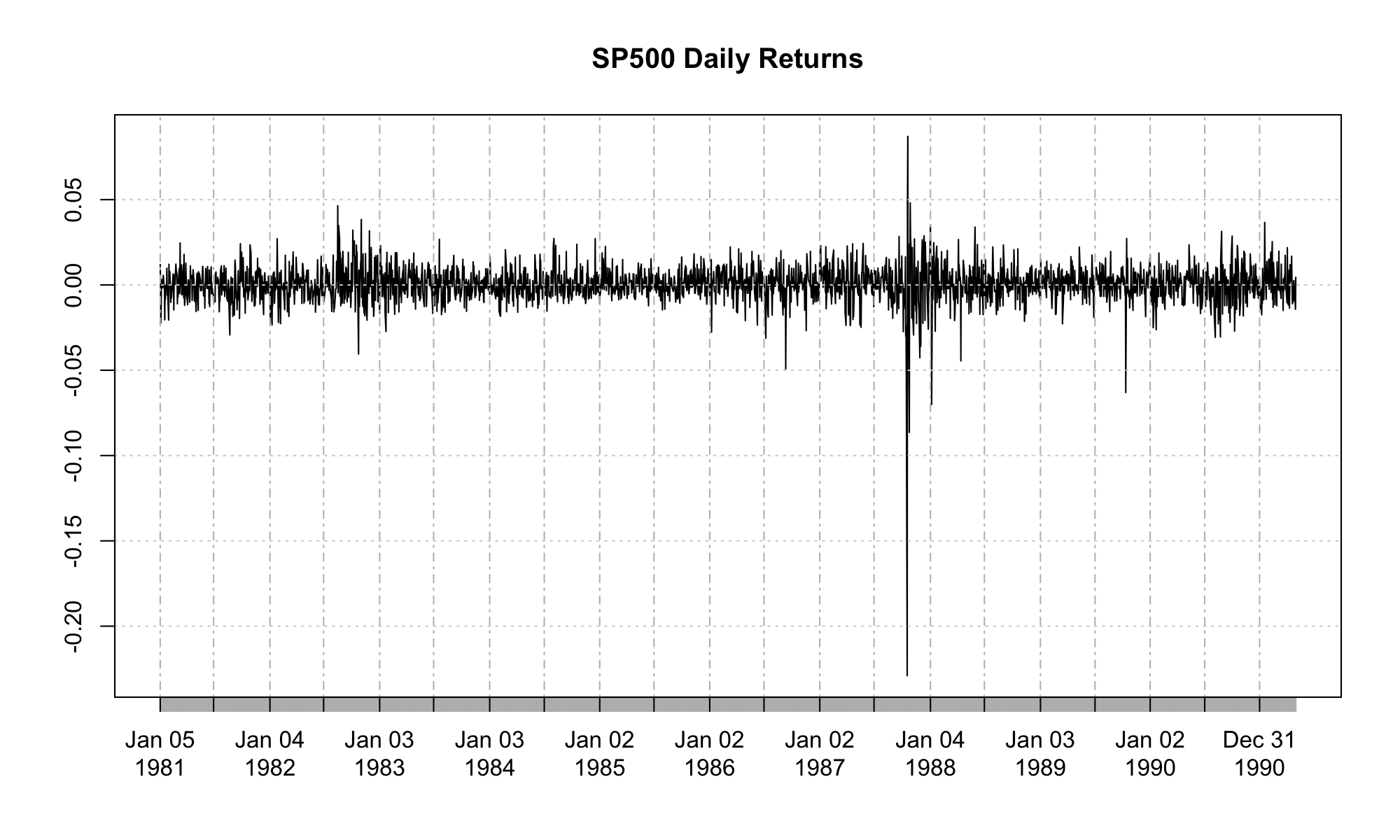
In the case of financial data, we will also view the observations \(y_1, y_2, \ldots, y_n\) as being ordered by time.

This is referred to as a time series.

Time Series Data Example¶

Histogram¶

Suppose we have dataset \(y_1, y_2, \ldots, y_n\) drawn from the same distribution \(F\).

We typically don’t know \(F\) and would like to estimate it with the data.

A simple estimate of \(F\) is obtained by a histogram.

A histogram:

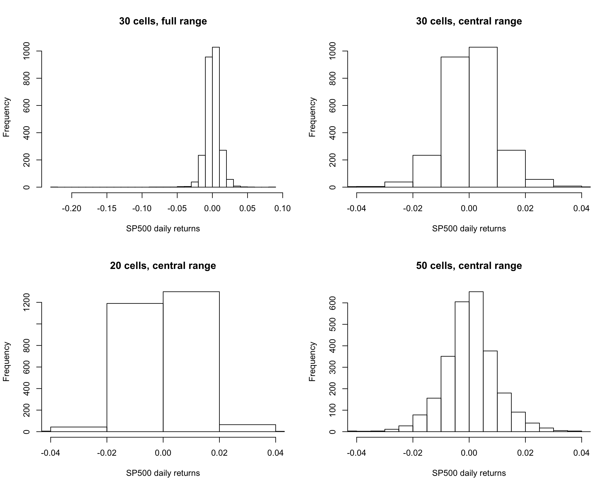
Divides the possible values of the random variable(s) \(y\) into \(K\) regions, called bins.

Counts the number of observations that fall into each bin.

Histogram of SP500 Daily Returns¶

Kernel Density Estimation¶

Histograms are crude estimators of density functions.

The kernel density estimator (KDE) is a better estimator.

A KDE uses a kernel, which is a probability density function symmetric about zero.

Often, the kernel is chosen to be a standard normal density.

The kernel has nothing to do with the true density of the data (i.e. choosing a normal kernel doesn’t mean the data is normally distributed).

Kernel Density Estimation¶

Given random variables \(Y_1, Y_2, \ldots, Y_n\), the KDE is

\[\widehat{f(y)} = \frac{1}{nb} \sum_{i=1}^n K\left(\frac{Y_i - y}{b} \right).\]

Kernel Density Estimation¶

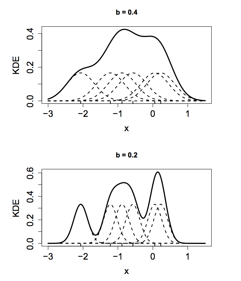
The KDE superimposes a density function (the kernel) over each data observation.

The bandwidth parameter \(b\) dictates the width of the kernel.

Larger values of \(b\) mean that the kernels of adjacent observations have a larger effect on the density estimate at a particular observation, \(y_i\).

In this fashion, \(b\) dictates the amount of data smoothing.

Illustration of KDE Estimator¶

This plot was taken directly from Ruppert (2011).

Kernel Density Bandwidth¶

Choosing \(b\) requires a tradeoff between bias and variance.

Small values of \(b\) detect fine features of the true density but permit a lot of random variation.

The KDE has high variance and low bias.

If \(b\) is too small, the KDE is undersmoothed or overfit - it adheres too closely to the data.

Kernel Density Bandwidth¶

Large values of \(b\) smooth over random variation but obscure fine details of the distribution.

The KDE has low variance and high bias.

If \(b\) is too large, the KDE is oversmoothed or underfit - it misses features of the true density.

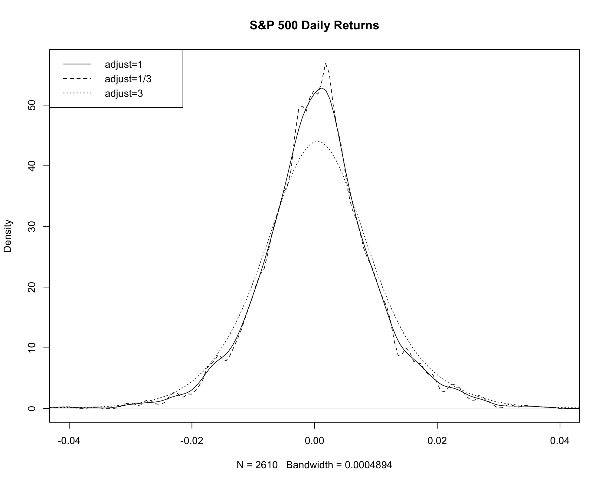
KDE of S&P 500 Daily Returns¶

The KDE of the S&P 500 returns suggests a density that resembles a normal distribution.

We can compare the KDE with a normal distribution with \(\mu = \hat{\mu}\) and \(\sigma^2 = \hat{\sigma}^2\), where

\[\hat{\mu} = \frac{1}{n}\sum_{i=1}^n y_i\]

\[\hat{\sigma}^2 = \frac{1}{n} \sum_{i=1}^n (y_i - \hat{\mu})^2.\]

KDE of S&P 500 Daily Returns¶

We can also compare the KDE with a normal distribution with \(\mu = \tilde{\mu}\) and \(\sigma^2 = \tilde{\sigma}^2\)

\[\tilde{\mu} = \text{median}\left(\{Y_i\}_{i=1}^n\right)\]

\[\begin{split}\tilde{\sigma}^2 & = \text{MAD}\left(\{Y_i\}_{i=1}^n\right) = \text{median}\left(\{|y_i - \tilde{\mu}|\}_{i=1}^n\right).\end{split}\]

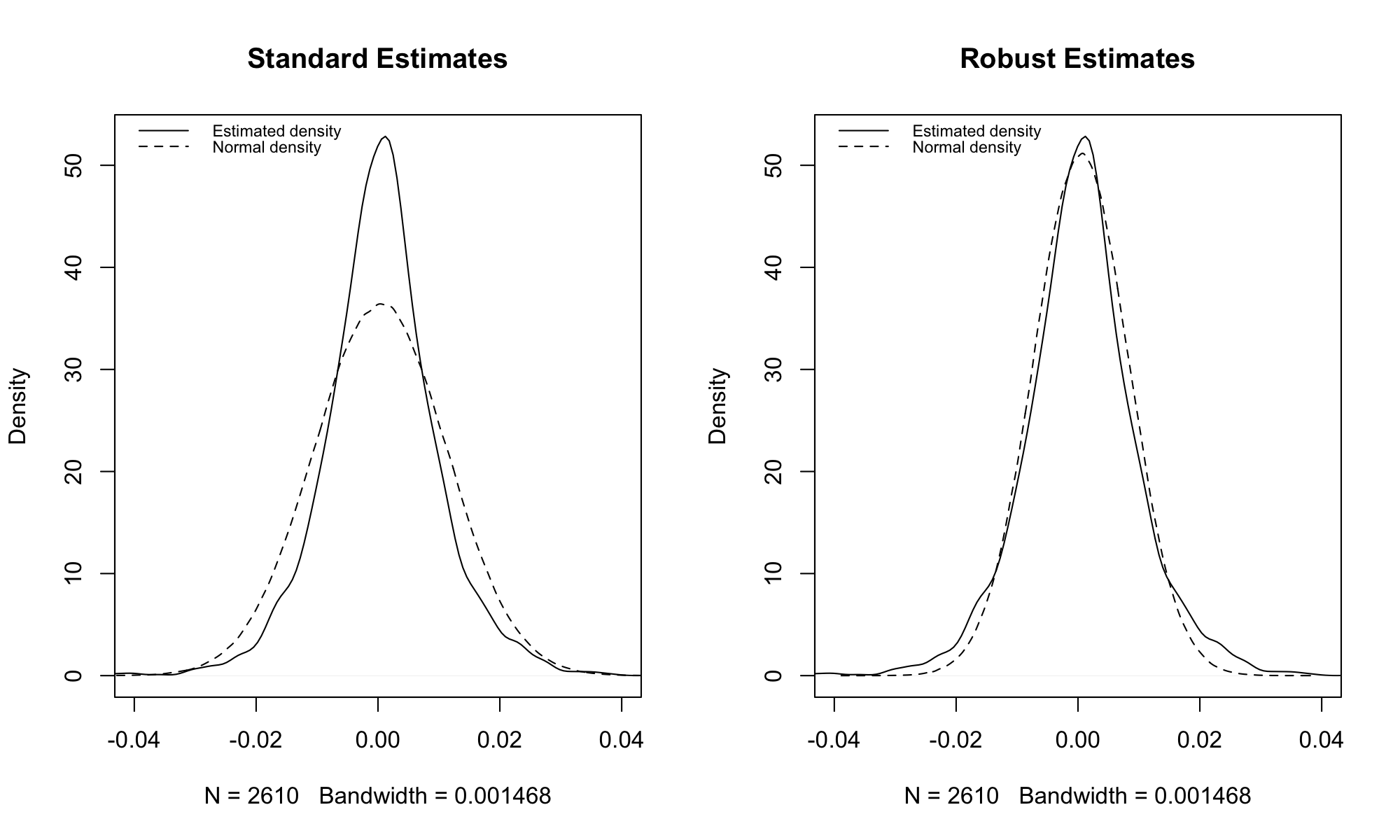
Comparison of KDE with Normal Densities¶

Outlying observations in the S&P 500 returns have great influence on the estimates \(\hat{\mu}\) and \(\hat{\sigma}^2\).

As a result, a \(N(\hat{\mu}, \hat{\sigma})\) deviates substantially from the KDE.

The median, \(\tilde{\mu}\), and median absolute deviation, \(\tilde{\sigma}^2\), are less sensitive (more robust) to outliers.

As a result, a \(N(\tilde{\mu}, \tilde{\sigma})\) deviates less from the KDE.

The fit is still not perfect - asset returns are often better approximated with a heavy tailed distribution, like the \(t\).