Moments
Moments
Given a random variable \(X\):
- The \(k\) -th moment of \(X\) is
\[E[X^k] = \int_{-\infty}^{\infty} x^k f(x) dx.\]
- The \(k\) -th central moment of \(X\) is
\[\mu_k = E\left[\left(X-E[X]\right)^k\right] =
\int_{-\infty}^{\infty} \left(x-E[X]\right)^k f(x) dx.\]
Moments
Some special cases for any random variable \(X\):
- The first moment of \(X\) is its mean.
- The first central moment of \(X\) is zero.
- The second central moment of \(X\) is its variance.
Sample Moments
Given realizations \(x_1, \ldots, x_n\) of a random variable \(X\),
- The moments of \(X\) can be approximated by replacing expectations with simple averages:
\[\hat{\mu}_k = \frac{1}{n} \sum_{i=1}^n (x_i - \bar{x})^k,
\,\,\,\,\,\, \text{where} \,\,\,\,\,\, \bar{x} = \frac{1}{n}
\sum_{i=1}^n x_i.\]
- For example, the sample variance is
\[\hat{\mu}_2 = \hat{\sigma}^2 = \frac{1}{n} \sum_{i=1}^n (x_i - \bar{x})^2.\]
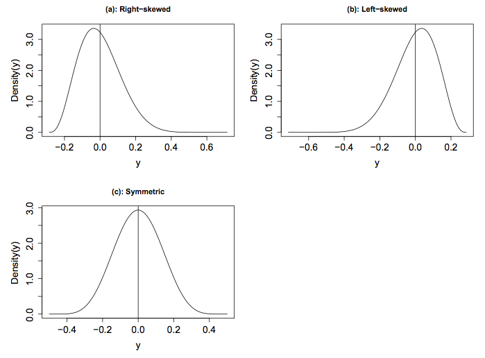
Skewness
Skewness measures the degree of asymmetry of a distribution.
- Formally, skewness is defined as
\[Sk = E\left[\left(\frac{X - E[X]}{\sigma}\right)^3\right] = \frac{\mu_3}{\sigma^3}.\]
- Zero skewness corresponds to a symmetric distribution.
- Positive skewness indicates a relatively long right tail.
- Negative skewness indicates a relatively long left tail.
Kurtosis
Kurtosis measures the extent to which probability is concentrated in the center and tails of a distribution rather than the “shoulders”.
- Formally, kurtosis is defined as
\[Kur = E\left[\left(\frac{X - E[Y]}{\sigma}\right)^4\right] =
\frac{\mu_4}{\sigma^4}.\]
- High values of kurtosis indicate heavy tails and low values indicate light tails.
Kurtosis
- For skewed distributions, kurtosis may measure both asymmetry and tail weight.
- For symmetric distributions, kurtosis only measures tail weight.
Kurtosis
The Kurtosis of a all normal distributions is 3.
- Excess Kurtosis, \(Kur - 3\), is a measure of the kurtosis of a distribution relative to that of a normal.
- If excess kurtosis is positive, the distribution has heavier tails than a normal.
- If excess kurtosis is negative, the distribution has lighter tails than a normal.
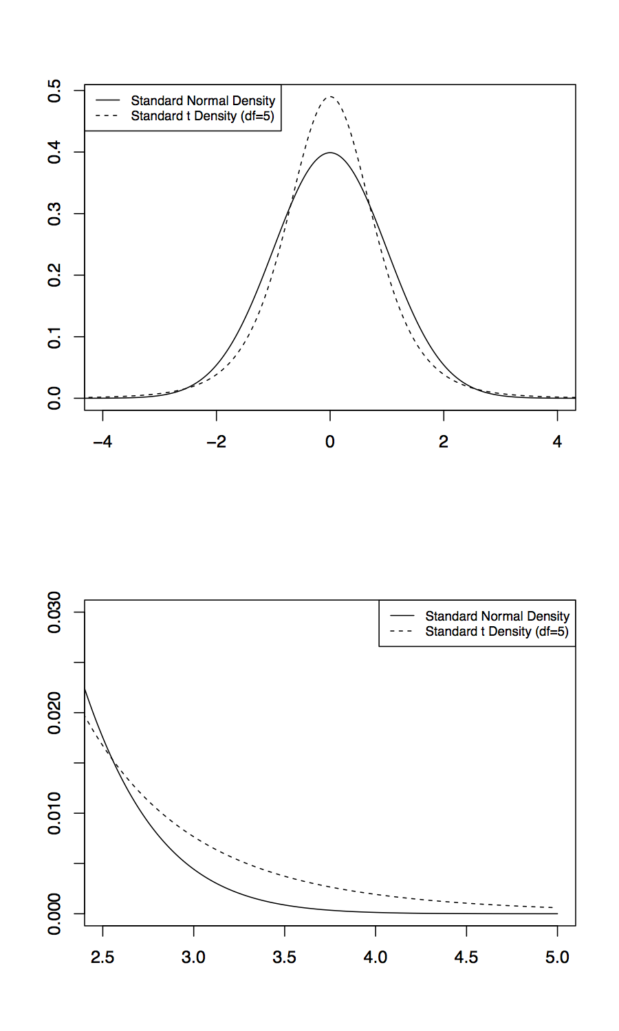
Kurtosis of \(t\)-Distribution
Let \(t_{\nu}\) denote a random variable that has a \(t\)-distribution with \(\nu\) degrees of freedom.
- The kurtosis of \(t_{\nu}\) exists only for \(\nu > 4\) and is equal to
\[Kur(t_{\nu}) = 3 + \frac{6}{\nu-4}.\]
- So, for a \(t_5\)-distribution, the kurtosis is 9.
- Clearly, as \(\nu \to \infty\), \(Kur(t_{\nu}) \to 3\), which is the kurtosis of a normal.
- This makes sense because \(t_{\nu} \to \mathcal{N}(0,1)\) as \(\nu \to \infty\).
Kurtosis Example
Sample Skewness and Kurtosis
Given realizations \(x_1, \ldots, x_n\) of a random variable \(X\), skewness and kurtosis can be approximated by
\[\widehat{SK} = \frac{1}{n} \sum_{i=1}^n \left(\frac{x_i -
\bar{x}}{\hat{\sigma}}\right)^3\]
\[\widehat{Kur} = \frac{1}{n} \sum_{i=1}^n \left(\frac{x_i -
\bar{x}}{\hat{\sigma}}\right)^4.\]
Sample Skewness and Kurtosis
Sample skewness and kurtosis can be used to diagnose normality.
- However, sample skewness and kurtosis are heavily influenced by outliers.
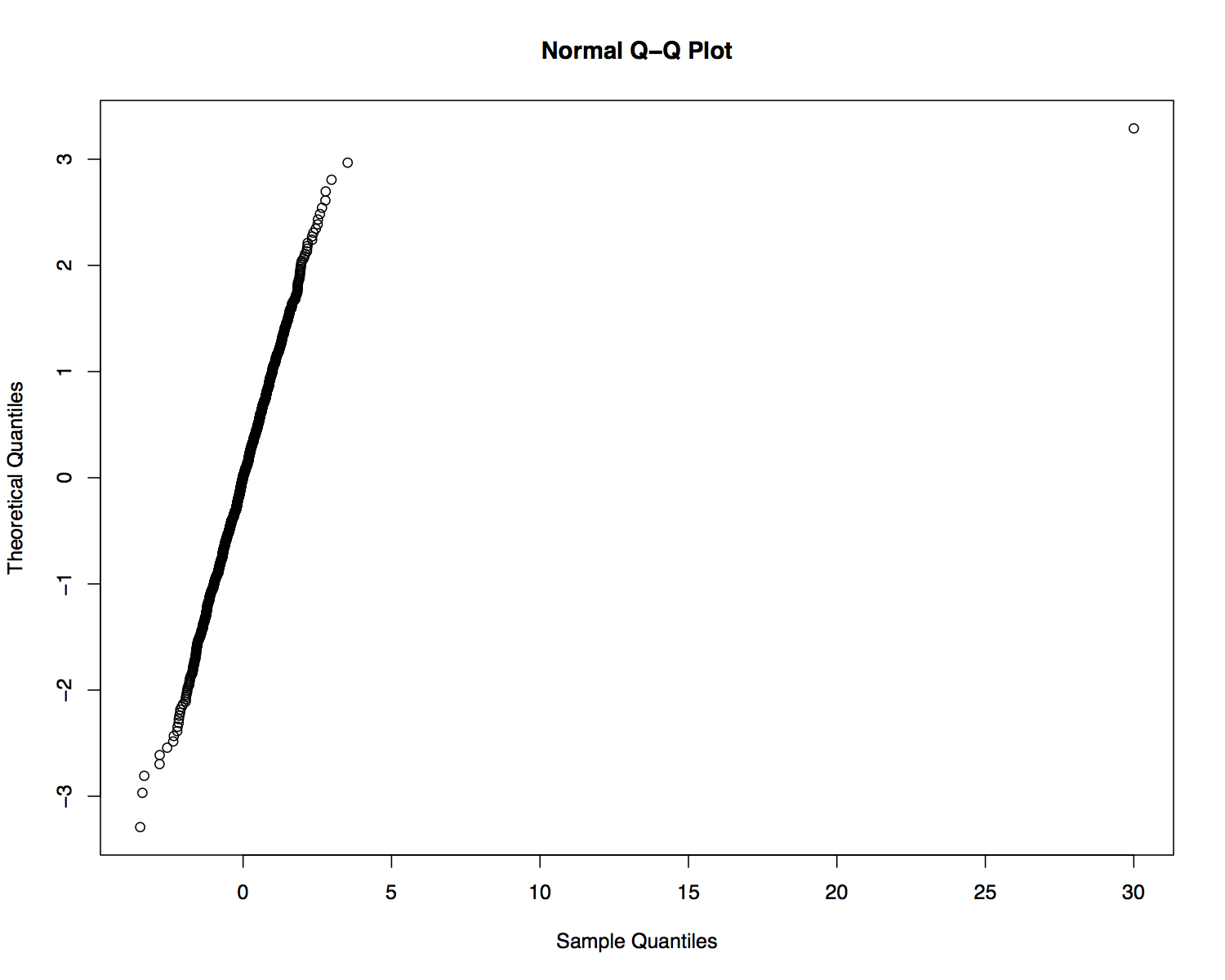
Sample Skewness and Kurtosis
- Consider a random sample of 999 values drawn from a \(\mathcal{N}(0,1)\) distribution.
- The sample skewness and kurtosis are 0.0072 and 3.17, respectively.
- These are close to the true values of 0 and 3.
- If one outlier equal to 30 is added to the dataset, the sample skewness and kurtosis become 10.48 and 231.05, respectively.
Sample Skewness and Kurtosis
Location, Scale and Shape Parameters
- A location parameter shifts a distribution to the right or left without changing the distribution’s variability or shape.
- A scale parameter changes the variability of a distribution without changing its location or shape.
- A parameter is a scale parameter if it increases by \(|a|\) when all data values are multiplied by \(a\).
- A shape parameter is any parameter that is not changed by location and scale parameters.
- Shape parameters dictate skewness and kurtosis.
Location, Scale and Shape Parameters
Examples of location, scale and shape parameters:
- The mean or median of any distribution are location parameters.
- The standard deviation (alternatively, variance) or median absolute deviation of any distribution are scale parameters.
- The degrees of freedom parameter of a \(t\) distribution is a shape parameter.