Heavy-Tailed Distributions
Heavy-Tailed Distributions
Observed data often do not conform to a Normal distribution.
- In many cases, extreme values are more likely than would be dictated by a Normal.
- This is especially true of financial data.
- In this lecture, we will study several examples of distributions with heavy tails, which assign higher probability to extreme values.
Generalized Error Distributions
Suppose that \(X\) follows a Generalized Error Distribution with shape parameter \(\nu: \,\, X \sim GED(\nu)\).
- Then for \(x \in (-\infty, \infty)\),
Generalized Error Distributions
- \(\lambda_{\nu}\) and \(\kappa(\nu)\) are constants and are chosen so that the density integrates to unity and has unit variance.
- The shape parameter \(\nu > 0\) determines tail weight.
Generalized Error Distributions
For many distributions, the scaling constants are simply a nuisance.
- We can focus attention on only the part of the function that relates to values of the random variable.
- Disregarding constants, we say that the density is proportional to:
- As \(x \to \infty\), \(-|x|^{\nu} \to -\infty\) faster for larger values of \(\nu\).
- This means that as \(x \to \infty\), \(f_{X}(x|\nu) \to 0\) faster for larger values of \(\nu\).
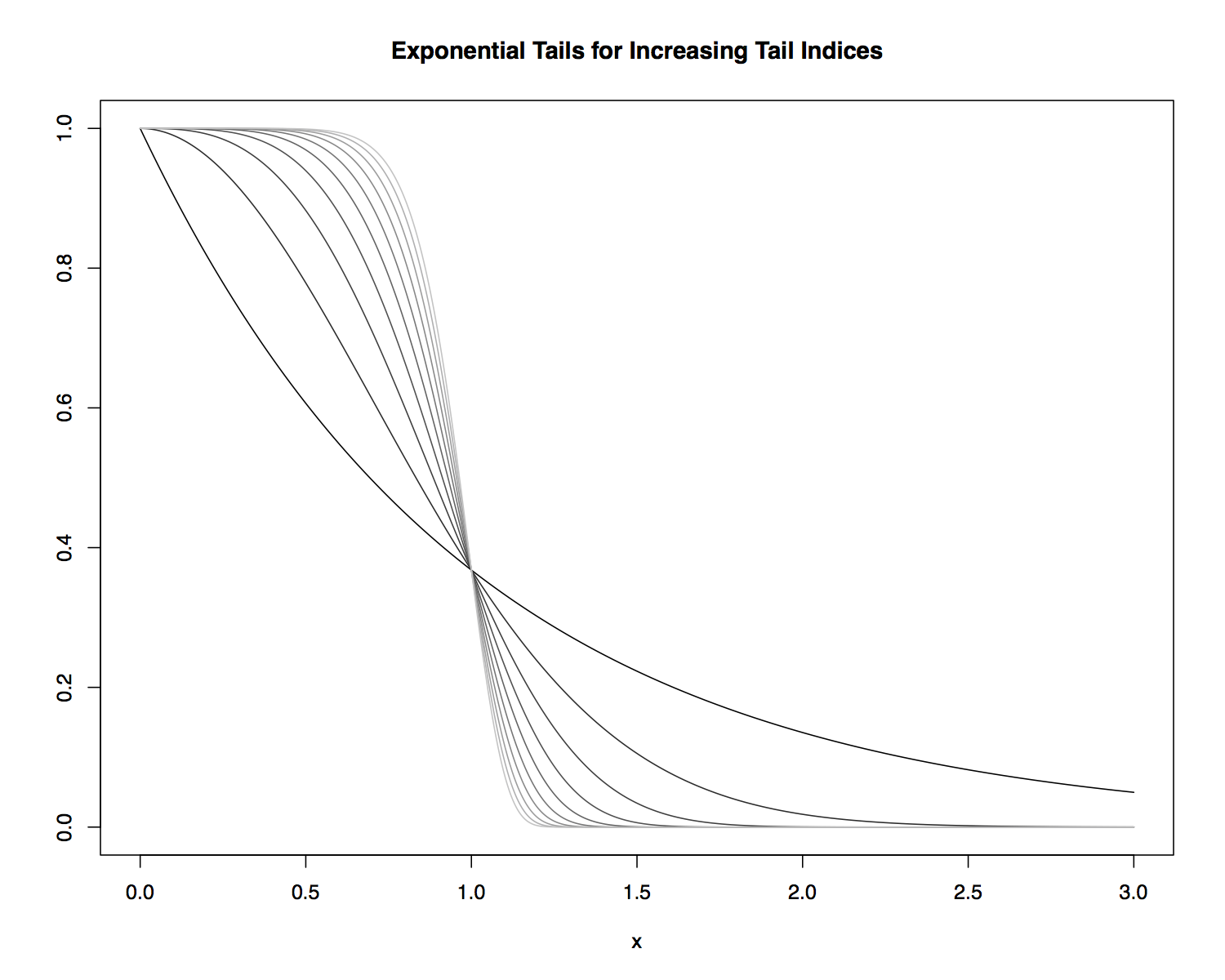
Exponential Tails
For generalized error distributions, larger values of \(\nu\) correspond to lighter tails and smaller values to heavier tails.
- We say that the generalized error distribution has exponential tails, since the tails diminish exponentially as \(x \to \infty\) and \(x \to -\infty\).
Exponential Tails
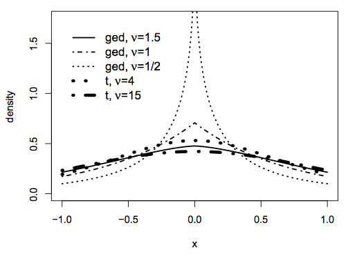
Generalized Error Distribution Examples
Special cases of generalized error distributions:
- \(\nu = 2\): \(\mathcal{N}(0,1)\).
- \(\nu = 1\): Double-exponential distribution.
- The double-exponential distribution has heavier tails than a standard normal since its shape parameter is smaller.
- Heavier tails that the double-exponential are obtained with \(\nu < 1\).
Power-Law Distributions
Suppose that \(X\) follows a Power-Law Distribution with shape parameter \(\alpha: \,\, X \sim PL(\alpha)\).
- Then for \(x \in (-\infty, \infty)\),
- \(A\) is chosen so that the density integrates to unity.
- \(\alpha > 0\), otherwise the density will integrate to \(\infty\).
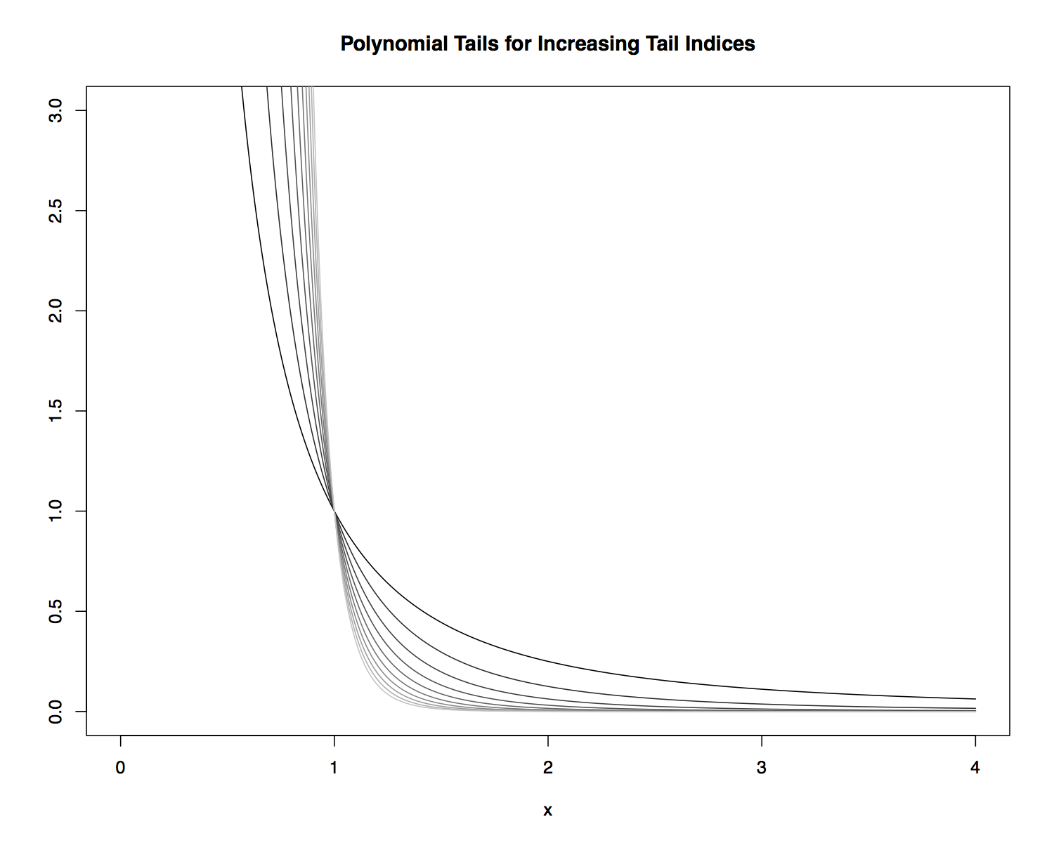
- The power-law distribution has a polynomial tail, because the tails diminish at a polynomial rate as \(x \to \infty\) and \(x \to -\infty\).
Polynomial Tails
The parameter \(\alpha\) is referred to as the tail index.
- As \(x \to \infty\), \(x^{-(1+\alpha)} \to 0\) faster for larger values of \(\alpha\).
- This means that larger values of \(\alpha\) correspond to lighter tails and smaller values to heavier tails.
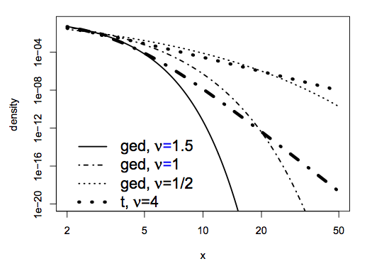
- A power-law distribution has heavier tails than a generalized error distribution:
Polynomial Tails
\(t\)-Distribution
The density of a \(t\) -distribution is
where
\(t\) -Distribution
Note that for large values of \(|y|\),
- This means the \(t\)-distribution has polynomial tails with tail index \(\nu\).
- Smaller values of \(\nu\) correspond to heavier tails.
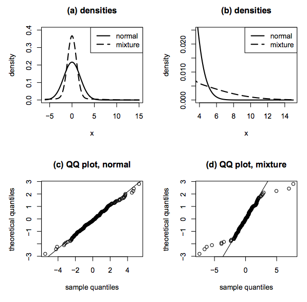
Discrete Mixtures
Consider a distribution that is 90% \(\mathcal{N}(0,1)\) and 10% \(\mathcal{N}(0,25)\).
- Generate \(X \sim \mathcal{N}(0,1)\).
- Generate \(U \sim Unif(0,1)\), with \(U\) independent of \(X\).
- Set \(Y = X\) if \(U < 0.9\).
- Set \(Y = 5X\) if \(U \geq 0.9\).
Discrete Mixtures
We say that \(Y\) follows a finite or discrete normal mixture distribution.
- Roughly 90% of the time it is drawn from a \(\mathcal{N}(0,1)\).
- Roughly 10% of the time it is drawn from a \(\mathcal{N}(0,25)\).
- The individual normal distributions are called the component distributions of \(Y\).
- This random variable could be used to model a market with two regimes: low volatility and high volatility.
Discrete Mixtures
The variance of \(Y\) is
- Consider \(Z \sim \mathcal{N}(0,\sqrt{3.4}) = \mathcal{N}(0,1.84)\).
- The distributions of \(Y\) and \(Z\) are very different.
- \(f_Y\) has much heavier tails than \(f_Z\).
- For example, the probability of observing the value 6 (3.25 standard deviations from the mean) is essentially zero for \(Z\).
- However, 10% of the time, the value 6 is only 6/5 = 1.2 standard deviations from the mean for \(Y\).
Continuous Mixtures
In general, \(Y\) follows a normal scale mixture distribution if
where
- \(\mu\) is a constant.
- \(Z \sim \mathcal{N}(0,1)\).
- \(U\) is a positive random variable giving the variance of each normal component.
- \(Z\) and \(U\) are independent.
Continuous Mixtures
- If \(U\) is continuous, \(Y\) follows a continuous scale mixture distribution.
- \(f_U\) is known as the mixing distribution.
- A finite normal mixture has exponential tails.
- A continuous normal mixture can have polynomial tails if the mixing distribution has heavy enough tails.
- The \(t\) -distribution is an example of a continuous normal mixture.