Maximum Likelihood Estimation¶

Estimating Parameters of Distributions¶

We almost never know the true distribution of a data sample.

We might hypothesize a family of distributions that capture broad characteristics of the data (locations, scale and shape).

However, there may be a set of one or more parameters of the distribution that we don’t know.

Typically we use the data to estimate the unknown parameters.

Joint Densities¶

Suppose we have a collection of random variables \({\bf Y} = (Y_1, \ldots, Y_n)'\).

We view a data sample of size \(n\) as one realization of each random variable: \({\bf y} = (y_1, \ldots, y_n)'\).

The joint cumulative density of \({\bf Y}\) is

\[\begin{split}F_{{\bf Y}}({\bf y}) & = P(Y_1 \leq y_1, \ldots, Y_n \leq y_n).\end{split}\]

Joint Densities¶

The joint probability density of \({\bf Y}\) is

\[\begin{split}f_{{\bf Y}}({\bf y}) & = \frac{\partial^n F_{{\bf Y}}({\bf y})}{\partial Y_1 \ldots \partial Y_n}.\end{split}\]

since

\[\begin{split}F_{{\bf Y}}({\bf y})& = \int_{-\infty}^{y_1}\ldots \int_{-\infty}^{y_n} f_{{\bf Y}}({\bf a}) \,\, da_1 \ldots da_n.\end{split}\]

Independence¶

When \(Y_1, \ldots, Y_n\) are independent of each other and have identical distributions:

We say that they are independent and identically distributed, or i.i.d.

When \(Y_1, \ldots, Y_n\) are i.i.d., they have the same marginal densities:

\[\begin{split}f_{Y_1}(y) & = \ldots = f_{Y_n}(y).\end{split}\]

Independence¶

Further, when \(Y_1, \ldots, Y_n\) are i.i.d.

\[\begin{split}f_{{\bf Y}}({\bf y}) & = f_{Y_1}(y_1) \cdot f_{Y_2}(y_2) \cdots f_{Y_n}(y_n) = \prod_{i=1}^n f_{Y_i}(y_i).\end{split}\]

This is analogous to the computation of joint probabilities.

For independent events \(A\), \(B\) and \(C\),

\[\begin{split}P(A \cap B \cap C) & = P(A)P(B)P(C).\end{split}\]

Maximum Likelihood Estimation¶

One of the most important and powerful methods of parameter estimation is maximum likelihood estimation. It requires

A data sample: \({\bf y} = (y_1, \ldots, y_n)'\).

A joint probability density:

\[\begin{split}f_{{\bf Y}}({\bf y}|{\bf \theta}) & = \prod_{i=1}^n f_{Y_i}(y_i|{\bf \theta}).\end{split}\]

where \({\bf \theta}\) is a vector of parameters.

Likelihood¶

\(f_{{\bf Y}}({\bf y}|{\bf \theta})\) is loosely interpreted as the probability of observing data sample \({\bf y}\), given a functional form for the density of \(Y_1, \ldots, Y_n\) and given a set of parameters \({\bf \theta}\).

We can reverse the notion and think of \({\bf y}\) as being fixed and \({\bf \theta}\) some unknown variable.

In this case we write \(\mathcal{L}({\bf \theta}|{\bf y}) = f_{{\bf Y}}({\bf y}|{\bf \theta})\).

We refer to \(\mathcal{L}({\bf \theta}|{\bf y})\) as the likelihood.

Fixing \({\bf y}\), maximum likelihood estimation chooses the value of \({\bf \theta}\) that maximizes \(\mathcal{L}({\bf \theta}|{\bf y}) = f_{{\bf Y}}({\bf y}|{\bf \theta})\).

Likelihood Maximization¶

Given \({\bf \theta} = (\theta_1, \ldots, \theta_p)'\), we maximize \(\mathcal{L}({\bf \theta}|{\bf y})\) by

Differentiating with respect to each \(\theta_i\), \(i = 1, \ldots, p\).

Setting the resulting derivatives equal to zero.

Solving for the values \(\hat{\theta}_i\), \(i = 1, \ldots, p\), that make all of the derivatives zero.

Log Likelihood¶

It is often easier to work with the logarithm of the likelihood function.

By the properties of logarithms

\[\begin{split}\ell({\bf \theta}|{\bf y}) & = \log\left(\mathcal{L}({\bf \theta}|{\bf y})\right)\end{split}\]

\[\begin{split}\qquad \enspace & = \log \left(f_{{\bf Y}}({\bf y}|{\bf \theta})\right)\end{split}\]

\[\begin{split}\qquad \enspace \qquad & = \log \left(\prod_{i=1}^n f_{Y_i}(y_i|{\bf \theta})\right)\end{split}\]

\[\begin{split}\qquad \qquad & = \sum_{i=1}^n \log\left(f_{Y_i}(y_i|{\bf \theta})\right).\end{split}\]

Log Likelihood¶

Maximizing \(\ell({\bf \theta}|{\bf y})\) is the same as maximizing \(\mathcal{L}({\bf \theta}|{\bf y})\) since \(\log\) is a monotonic transformation.

A derivative of \(\mathcal{L}\) will involve many chain-rule products, whereas a derivative of \(\ell\) will simply be a sum of derivatives.

MLE Example¶

Suppose we have a dataset \({\bf y} = (y_1, \ldots, y_n)\), where \(Y_1, \ldots, Y_n \stackrel{i.i.d.}{\sim} \mathcal{N}(\mu, \sigma^2)\).

We will assume \(\mu\) is unknown and \(\sigma\) is known.

So, \({\bf \theta} = \mu\) (it is a single value, rather than a vector).

MLE Example¶

The likelihood is

\[\begin{split}\mathcal{L}(\mu|{\bf y}) & = f_{{\bf Y}}({\bf y}|\mu) \qquad \qquad \qquad \qquad \qquad \qquad\end{split}\]

\[\begin{split}& = \prod_{i=1}^n f_{Y_i}(y_i|\mu) \qquad \qquad \qquad \qquad\end{split}\]

\[\begin{split}\quad & = \prod_{i=1}^n \frac{1}{\sqrt{2\pi \sigma^2}} \exp \left\{-\frac{1}{2} \frac{(y_i - \mu)^2}{\sigma^2} \right\}\end{split}\]

\[\begin{split}\qquad \enspace & = \frac{1}{(2\pi \sigma^2)^{n/2}} \exp \left\{-\frac{1}{2 \sigma^2} \sum_{i=1}^n (y_i - \mu)^2 \right\}.\end{split}\]

MLE Example¶

The log likelihood is

\[\begin{split}\ell(\mu|{\bf y}) & = -\frac{n}{2} \log(2\pi) - \frac{n}{2} \log(\sigma^2) - \frac{1}{2 \sigma^2} \sum_{i=1}^n (y_i - \mu)^2.\end{split}\]

MLE Example¶

The MLE, \(\hat{\mu}\), is the value that sets \(\frac{d}{d \mu} \ell(\mu|{\bf y}) = 0\):

\[\frac{d}{d \mu} \ell(\mu|{\bf y}) \bigg|_{\hat{\mu}} = \frac{1}{\sigma^2} \sum_{i=1}^n (y_i - \hat{\mu}) = 0\]

\[\Rightarrow \sum_{i=1}^n (y_i - \hat{\mu}) = 0\]

\[\Rightarrow \sum_{i=1}^n \hat{\mu} = \sum_{i=1}^n y_i\]

\[\Rightarrow \hat{\mu} = \bar{y} = \frac{1}{n} \sum_{i=1}^n y_i.\]

MLE Example: \(n=1\), Unknown \(\mu\)¶

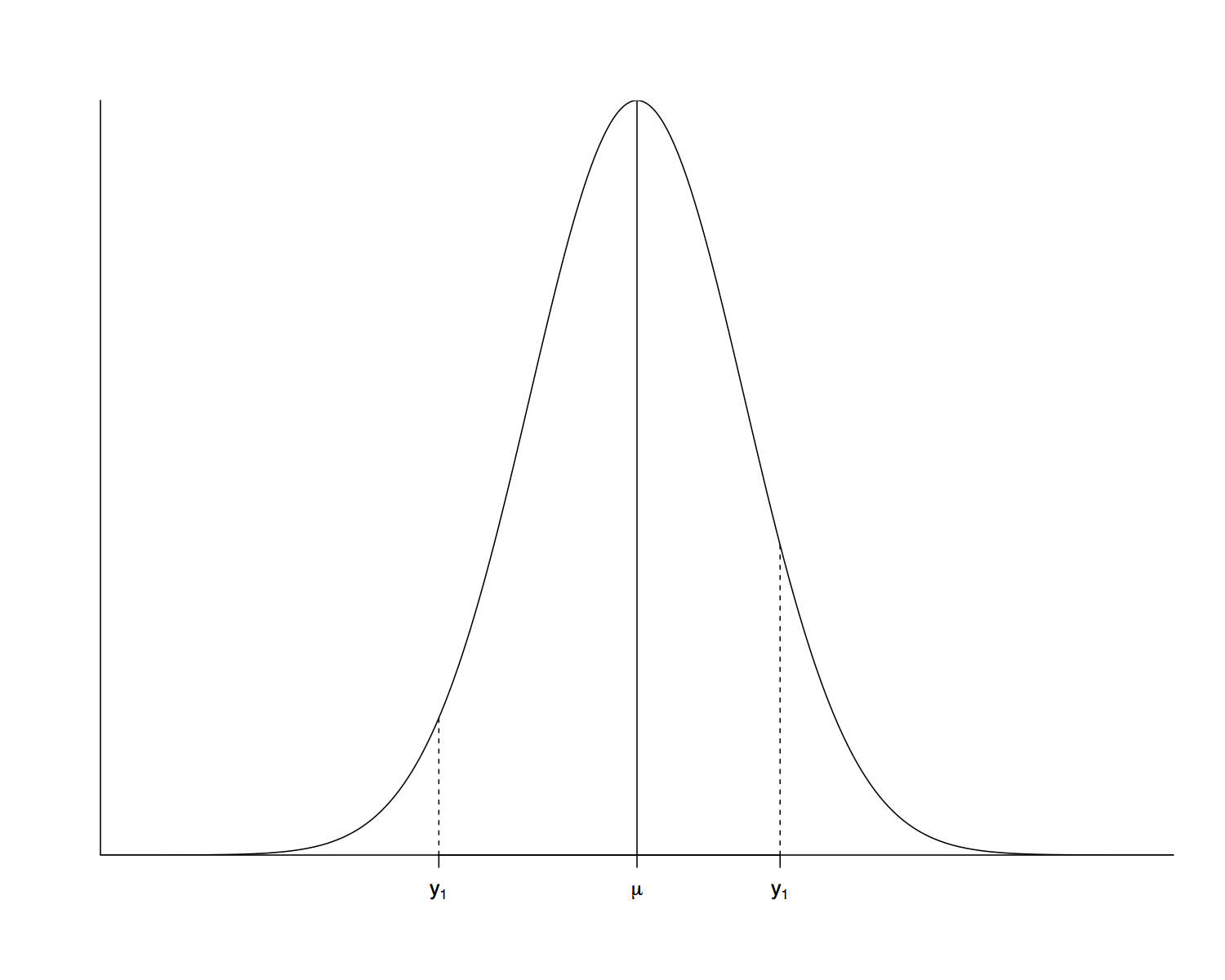
Suppose we have only one observation: \(y_1\).

If we specialize the previous result:

\[\begin{split}\hat{\mu} & = y_1.\end{split}\]

The density \(f_{Y_1}(y_1|\mu)\) gives the probability of observing some data value \(y_1\), conditional on some known parameter \(\mu\).

This is a normal distribution with mean \(\mu\) and variance \(\sigma^2\).

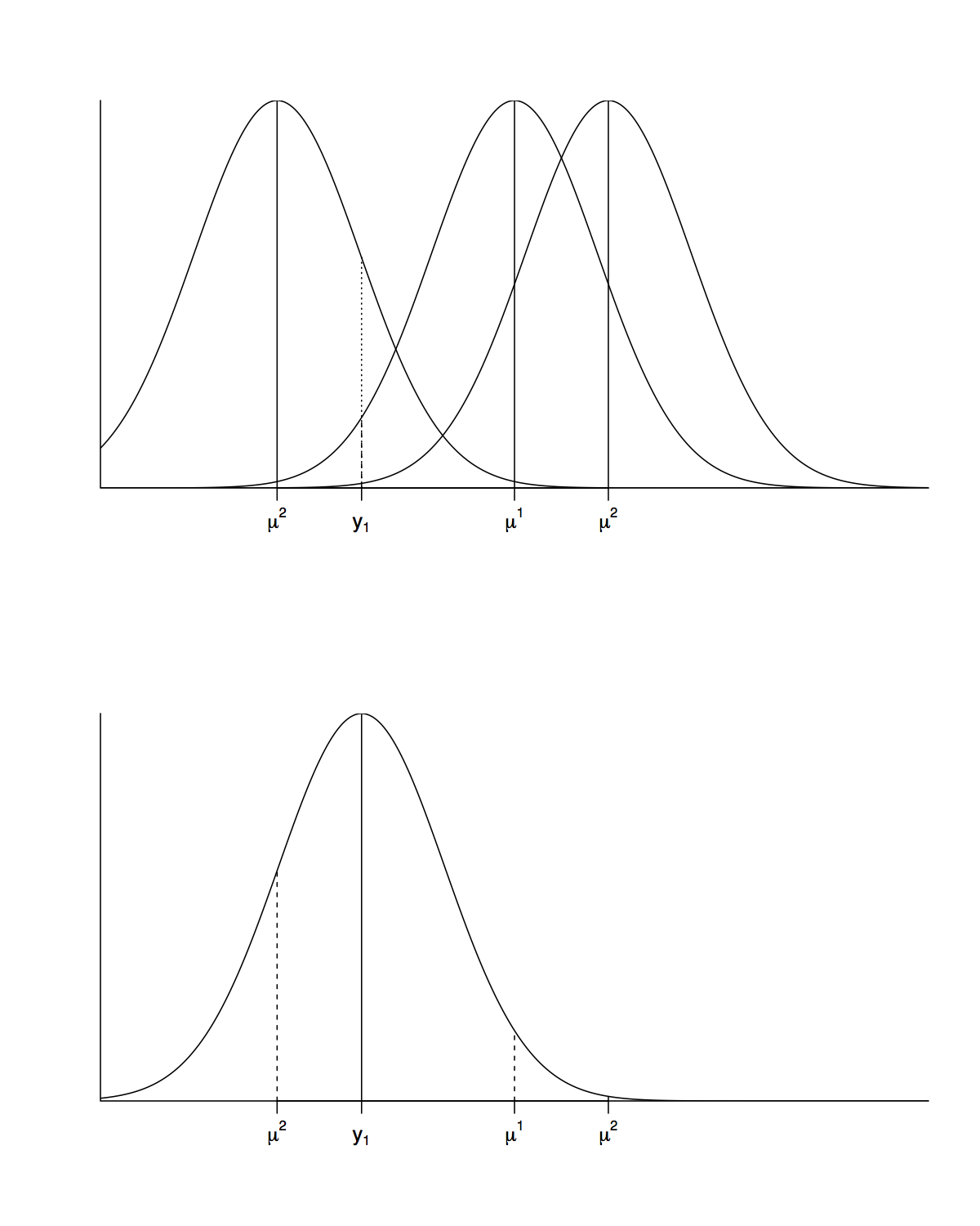
MLE Example: \(n=1\), Unknown \(\mu\)¶

The likelihood \(\mathcal{L}(\mu|y_1)\) gives the probability of \(\mu\), conditional on some observed data value \(y_1\).

This is a normal distribution with mean \(y_1\) and variance \(\sigma^2\).

MLE Example: \(n=1\)¶

MLE Example: \(n=1\), Unknown \(\mu\)¶

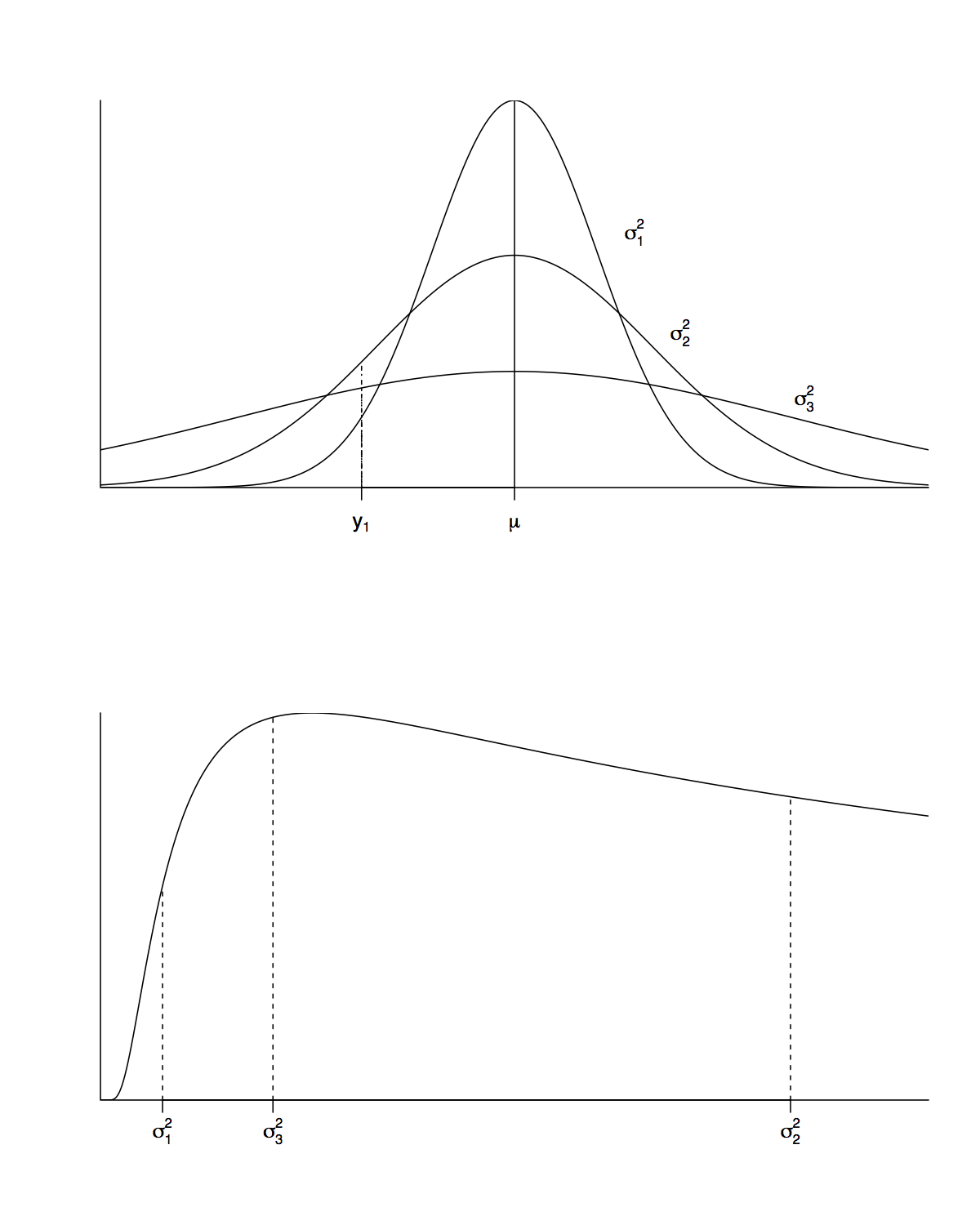
MLE Example: \(n=1\), Unknown \(\sigma\)¶

Let’s continue with the assumption of one data observation, \(y_1\).

If \(\mu\) is known but \(\sigma\) is unknown, the density of the data, \(y_1\), is still normal.

However, the likelihood is

\[\mathcal{L}(\sigma^2|y_1) = \frac{\alpha}{\sigma^2} \exp\left\{-\frac{\beta}{\sigma^2}\right\}\]

\[\alpha = \frac{1}{\sqrt{2\pi}}, \qquad \beta = \frac{(y_1-\mu)^2}{2}.\]

The likelihood for \(\sigma^2\) is not normal, but inverse gamma.

MLE Example: \(n=1\), Unknown \(\sigma\)¶

MLE Accuracy¶

Maximum likelihood estimation results in estimates of true unknown parameters.

What is the probability that our estimates are identical to the true population parameters?

Our estimates are imprecise and contain error.

We would like to quantify the precision of our estimates with standard errors.

We will use the Fisher Information to compute standard errors.

Fisher Information¶

Suppose our likelihood is a function of a single parameter, \(\theta\): \(\mathcal{L}(\theta|{\bf y})\).

The Fisher Information is

\[\begin{split}\mathcal{I}(\theta) & = - E\left[\frac{d^2}{d \theta^2} \ell(\theta|{\bf y}) \right].\end{split}\]

The observed Fisher Information is

\[\begin{split}\widetilde{\mathcal{I}}(\theta) & = - \frac{d^2}{d \theta^2} \ell(\theta|{\bf y}).\end{split}\]

Fisher Information¶

Observed Fisher Information does not take an expectation, which may be difficult to compute.

Since \(\ell(\theta|{\bf y})\) is often a sum of many terms, \(\widetilde{\mathcal{I}}(\theta)\) will converge to \(\mathcal{I}(\theta)\) for large samples.

MLE Central Limit Theorem¶

Under certain conditions, a central limit theorem holds for the MLE, \(\hat{\theta}\).

For infinitely large samples \({\bf y}\),

\[\hat{\theta} \sim \mathcal{N}(\theta, \mathcal{I}(\theta)^{-1}).\]

For large samples, \(\hat{\theta}\) is normally distributed regardless of the distribution of the data, \({\bf y}\).

MLE Central Limit Theorem¶

\(\hat{\theta}\) is also normally distributed for large samples even if \(\mathcal{L}(\theta|{\bf y})\) is some other distribution.

Hence, for large samples,

\[\begin{split}Var(\hat{\theta}) & = \frac{1}{\mathcal{I}(\theta)} \qquad \Rightarrow \qquad Std(\hat{\theta}) = \frac{1}{\sqrt{\mathcal{I}(\theta)}}.\end{split}\]

MLE Standard Errors¶

Since we don’t know the true \(\theta\), we approximate

\[\begin{split}Std(\hat{\theta}) & \approx \frac{1}{\sqrt{\mathcal{I}(\hat{\theta})}}.\end{split}\]

Alternatively, to avoid computing the expectation, we could use the approximation

\[\begin{split}Std(\hat{\theta}) & \approx \frac{1}{\sqrt{\widetilde{\mathcal{I}}(\hat{\theta})}}.\end{split}\]

MLE Standard Errors¶

In reality, we never have an infinite sample size.

For finite samples, these values are approximations of the standard error of \(\hat{\theta}\).

MLE Variance Example¶

Let’s return to the example where \(Y_1, \ldots, Y_n \stackrel{i.i.d.}{\sim} \mathcal{N}(\mu, \sigma^2)\), with known \(\sigma\).

The log likelihood is

\[\begin{split}\ell(\mu|{\bf y}) & = -\frac{n}{2} \log(2\pi) - \frac{n}{2} \log(\sigma^2) - \frac{1}{2 \sigma^2} \sum_{i=1}^n (y_i - \mu)^2.\end{split}\]

The resulting derivatives are

\[\begin{split}\frac{\partial \ell(\mu|{\bf y})}{\partial \mu} & = \frac{1}{\sigma^2} \sum_{i=1}^n (y_i - \mu), \qquad \frac{\partial^2 \ell(\mu|{\bf y})}{\partial \mu^2} = -\frac{n}{\sigma^2}.\end{split}\]

MLE Variance Example¶

In this case the Fisher Information is identical to the observed Fisher Information:

\[\begin{split}\mathcal{I}(\mu) & = -E\left[-\frac{n}{\sigma^2}\right] = \frac{n}{\sigma^2} = \widetilde{\mathcal{I}}(\mu).\end{split}\]

Since \(\mathcal{I}(\mu)\) doesn’t depend on \(\mu\), we don’t need to resort to an approximation with \(\hat{\mu} = \bar{{\bf y}}\).

The result is

\[\begin{split}Std(\hat{\mu}) & = \frac{1}{\sqrt{\mathcal{I}(\mu)}} = \frac{\sigma}{\sqrt{n}}.\end{split}\]