Moving Average Processes
\(MA(1)\)
Given white noise \(\{\varepsilon_t\}\), consider the process
where \(\mu\) and \(\theta\) are constants.
- This is a first-order moving average or \(MA(1)\) process.
\(MA(1)\) Mean and Variance
The mean of the first-order moving average process is
\(MA(1)\) Autocovariances
\(MA(1)\) Autocovariances
- If \(j = 0\)
- If \(j = 1\)
- If \(j > 1\), all of the expectations are zero:
\(MA(1)\) Stationarity
Since the mean and autocovariances are independent of time, an \(MA(1)\) is weakly stationary.
- This is true for all values of \(\theta\).
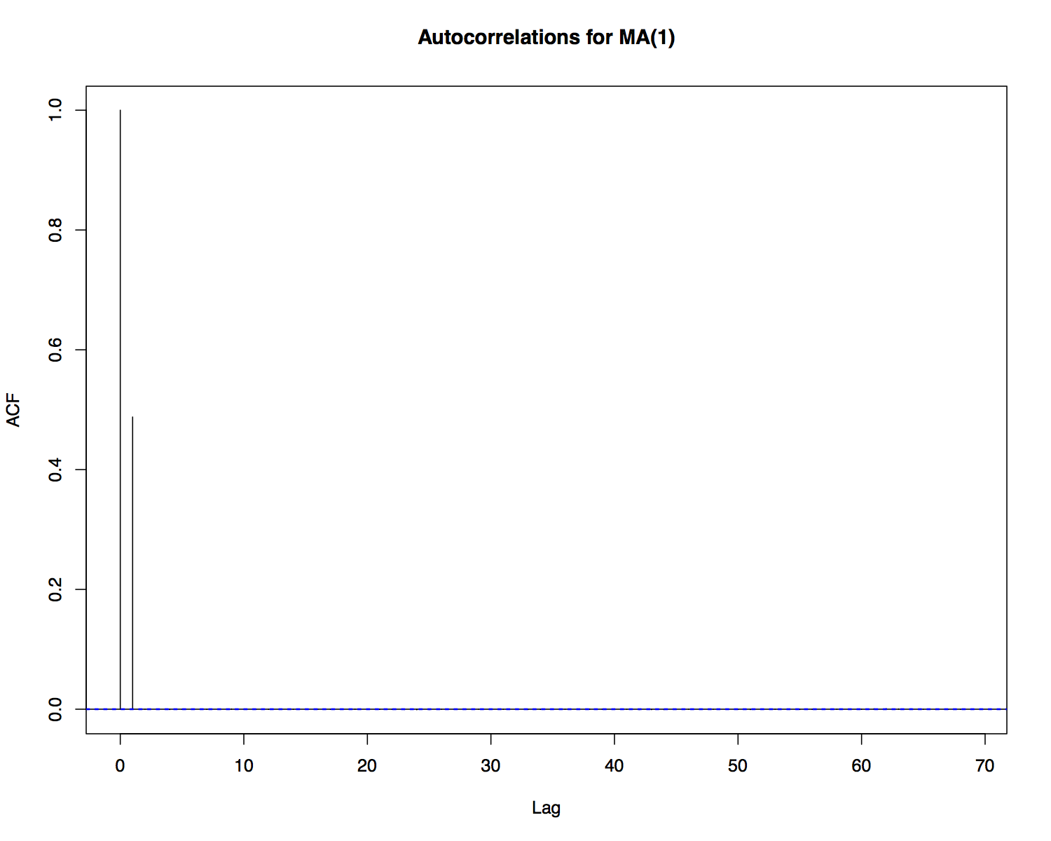
\(MA(1)\) Autocorrelations
The autocorrelations of an \(MA(1)\) are
- \(j = 0\): \(\hspace{0.7in} \rho_0 = 1\) (always).
- \(j = 1\):
- \(j > 1\): \(\hspace{0.72in} \rho_j = 0\).
- If \(\theta > 0\), first-order lags of \(Y_t\) are positively autocorrelated.
- If \(\theta < 0\), first-order lags of \(Y_t\) are negatively autocorrelated.
\(MA(1)\) Autocorrelations
\(MA(q)\)
A \(q\) th-order moving average or \(MA(q)\) process is
where \(\mu, \theta_1, \ldots, \theta_q\) are any real numbers.
\(MA(q)\) Mean
As with the \(MA(1)\):
\(MA(q)\) Autocovariances
- For \(j > q\), all of the products result in zero expectations: \(\gamma_j = 0\), for \(j > q\).
\(MA(q)\) Autocovariances
- For \(j = 0\), the squared terms result in nonzero expectations, while the cross products lead to zero expectations:
\(MA(q)\) Autocovariances
- For \(j = \{1,2,\ldots,q\}\), the nonzero expectation terms are
The autocovariances can be stated concisely as
where \(\theta_0 = 1\).
\(MA(q)\) Autocorrelations
The autocorrelations can be stated concisely as
where \(\theta_0 = 1\).
\(MA(2)\) Example
For an \(MA(2)\) process
Estimating \(MA\) Models
Estimation of an \(MA\) model is done via maximum likelihood.
- For an \(MA(q)\) model, one would first specify a joint likelihood for the parameters \(\{\theta_1, \ldots, \theta_q, \mu, \sigma^2\}\).
- Taking derivatives of the log likelihood with respect to each of the parameters would result in a system of equations that could be solved for the MLEs: \(\{\hat{\theta}_1, \ldots, \hat{\theta}_q, \hat{\mu}, \hat{\sigma}^2\}\).
- The exact likelihood is a bit cumbersome and maximization requires specialized numerical methods.
- The MLEs can be obtained with the \(\mathtt{arima}\) function in \(\mathtt{R}\).
Which \(MA\)?
How do we know if an \(MA\) model is appropriate and which \(MA\) model to fit?
- For an \(MA(q)\), we know that \(\gamma_j = 0\) for \(j > q\).
- We should only fit an \(MA\) model if the autocorrelations drop to zero for all \(j > q\) for some value \(q\).
- The \(\mathtt{acf}\) function in \(\mathtt{R}\) can be used to compute empirical autocorrelations of the data.
- The appropriate \(q\) can then be obtained from the empirical ACF.
Which \(MA\)?
- After fitting an \(MA\) model, we can examine the residuals.
- The \(\mathtt{acf}\) function can be used to compute empirical autocorrelations of the residuals.
- If the residuals are autocorrelated, the model is not a good fit. Consider changing the order of the \(MA\) or using another model.
Which \(MA\)?
The \(\mathtt{auto.arima}\) function in \(\mathtt{R}\) estimates a range of \(MA(q)\) models and selects the one with the best fit.
- \(\mathtt{auto.arima}\) uses the Akaike Information Criterion (AIC) or the Bayesian Information Criterion (BIC) to select the model.
- Minimizing AIC and BIC amounts to minimizing the sum of squared residuals, with a penalty term that is related to the number of model parameters.