Autoregressive Processes
\(AR(1)\) Process
Given white noise \(\{\varepsilon_t\}\), consider the process
where \(c\) and \(\phi\) are constants.
- This is a first-order autoregressive or \(AR(1)\) process.
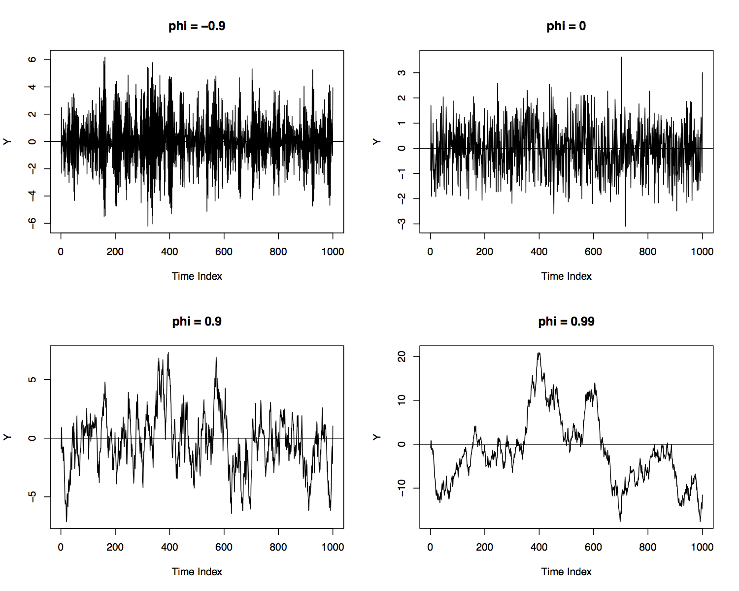
- \(\phi\) can be thought of as a memory or feedback parameter and introduces serial correlation in \(Y_t\).
- When \(\phi = 0\), \(Y_t\) is white noise with drift - it has no memory or serial correlation.
Recursive Substitution of \(AR(1)\)
Applying recursive substitution:
Recursive Substitution of \(AR(1)\)
- The infinite recursive substitution can only be performed if \(|\phi| < 1\).
Expectation of \(AR(1)\)
Assume \(Y_t\) is weakly stationary: \(|\phi| < 1\).
A Useful Property
If \(Y_t\) is weakly stationary,
- That is, for \(j \geq 1\), \(Y_{t-j}\) is a function of lagged values of \(\varepsilon_t\) and not \(\varepsilon_t\) itself.
- As a result, for \(j \geq 1\)
Variance of \(AR(1)\)
Given that \(\mu = c/(1-\phi)\) for weakly stationary \(Y_t\):
Squaring both sides and taking expectations:
Autocovariances of \(AR(1)\)
For \(j \geq 1\),
Autocorrelations of \(AR(1)\)
The autocorrelations of an \(AR(1)\) are
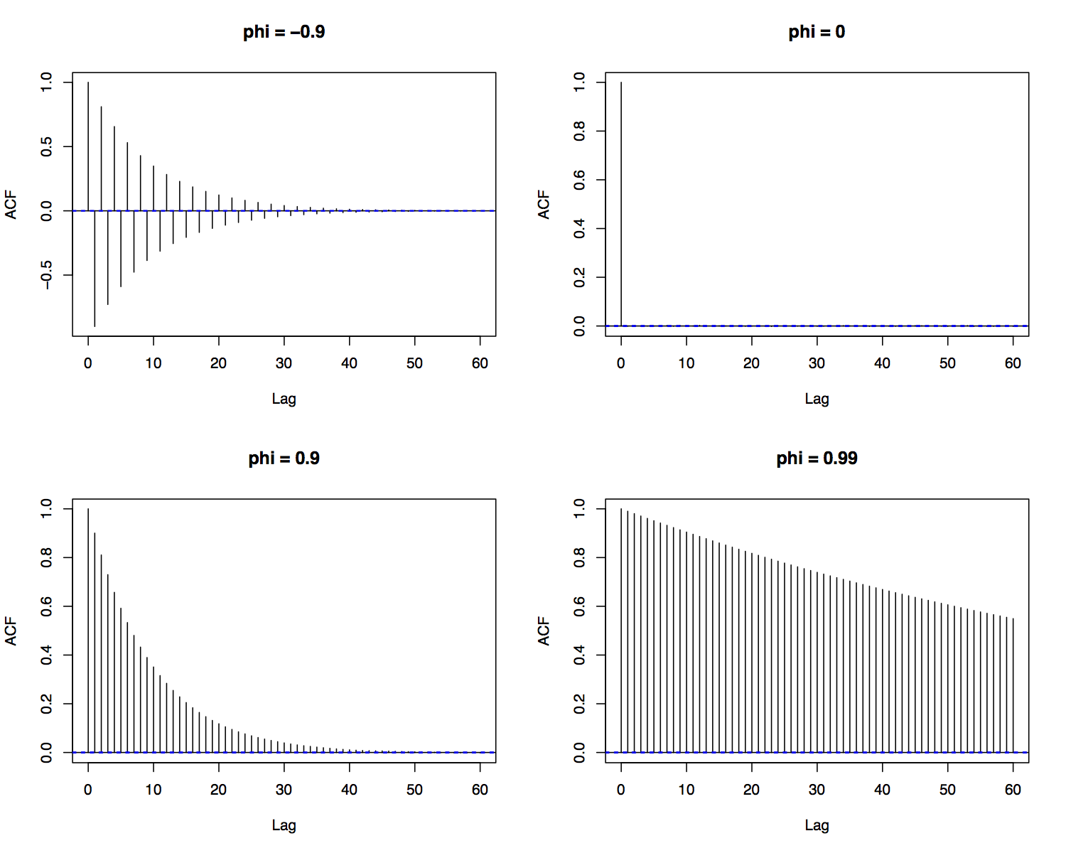
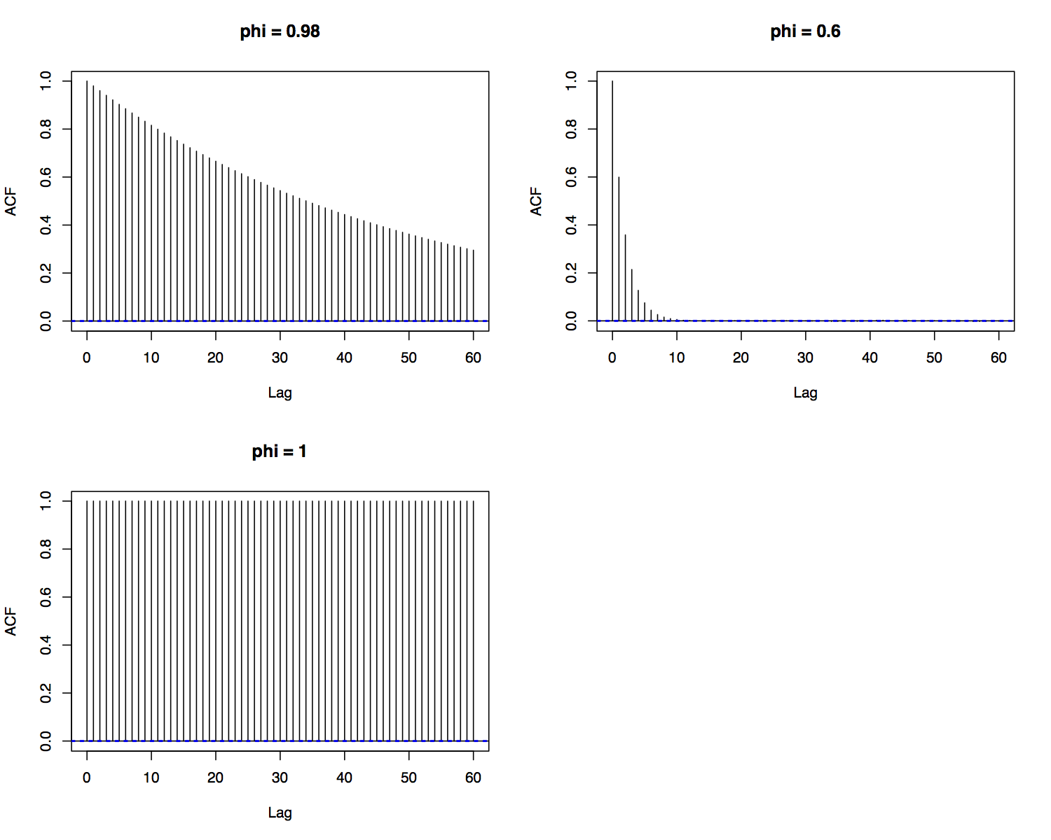
- Since we assumed \(|\phi| < 1\), the autocorrelations decay exponentially as \(j\) increases.
- Note that if \(\phi \in (-1,0)\), the autocorrelations decay in an oscillatory fashion.
Examples of \(AR(1)\) Processes
\(AR(1)\) Autocorrelations
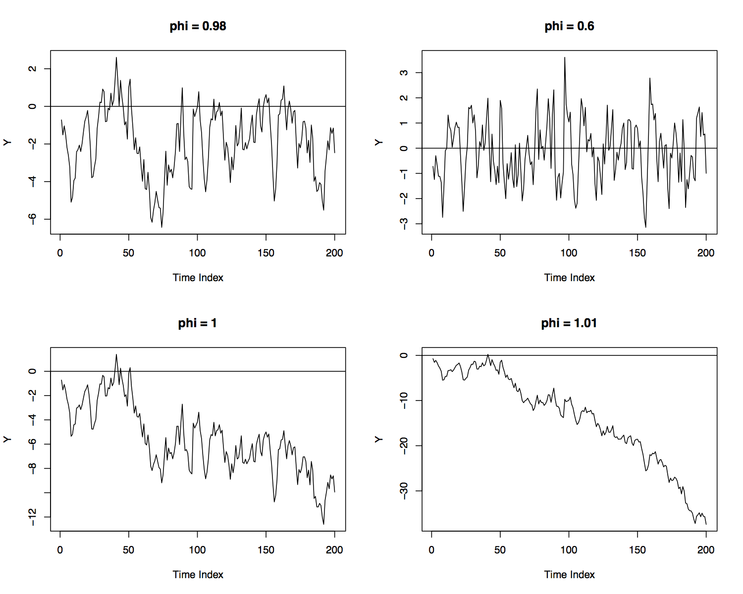
Random Walk
Suppose \(\phi = 1\):
- Clearly \(E[Y_t] = tc + Y_0\), which is not independent of time.
- \(Var(Y_t) = t\sigma^2\), which increases linearly with time.
Explosive \(AR(1)\)
When \(|\phi| > 1\), the autoregressive process is explosive.
- Recall that \(Y_t = \frac{c}{1-\phi} + \sum_{i=0}^{\infty} \phi^i \varepsilon_{t-i}\).
- Now \(|\phi^i|\) increases with \(i\) rather than decay.
- Past values of \(\varepsilon_{t-i}\) contribute greater amounts to \(Y_t\) as \(i\) increases.
Examples of \(AR(1)\) Processes
\(AR(1)\) Autocorrelations
\(AR(p)\) Process
Given white noise \(\{\varepsilon_t\}\), consider the process
where \(c\) and \(\{\phi\}_{i=1}^p\) are constants.
- This is a \(p\) th-order autoregressive or \(AR(p)\) process.
Expectation of \(AR(p)\)
Assume \(Y_t\) is weakly stationary.
Autocovariances of \(AR(p)\)
Given that \(\mu = c/(1-\phi_1 - \ldots - \phi_p)\) for weakly stationary \(Y_t\):
Autocovariances of \(AR(p)\)
Thus,
Autocovariances of \(AR(p)\)
For \(j = 0, 1, \ldots, p\), System (1) is a system of \(p+1\) equations with \(p+1\) unknowns: \(\{\gamma_j\}_{j=0}^p\).
- \(\{\gamma_j\}_{j=0}^p\) can be solved for as functions of \(\{\phi_j\}_{j=1}^p\) and \(\sigma^2\).
- It can be shown that \(\{\gamma_j\}_{j=0}^p\) are the first \(p\) elements of the first column of \(\sigma^2 [I_{p^2} - \Phi \otimes \Phi]^{-1}\), where \(\otimes\) denotes the Kronecker product.
- \(\{\gamma_j\}_{j=p+1}^{\infty}\) can then be determined using prior values of \(\gamma_j\) and \(\{\phi_j\}_{j=1}^p\).
Autocorrelations of \(AR(p)\)
Dividing the autocovariances by \(\gamma_0\),
Estimating \(AR\) Models
Ideally, estimation of an \(AR\) model is done via maximum likelihood.
- For an \(AR(p)\) model, one would first specify a joint likelihood for the parameters \({\phi_1, \ldots, \phi_p, c, \sigma^2}\).
- Taking derivatives of the log likelihood with respect to each of the parameters would result in a system of equations that could be solved for the MLEs: \({\hat{\phi}_1, \ldots, \hat{\phi}_p, \hat{c}, \hat{\sigma}^2}\).
Estimating \(AR\) Models
- The exact likelihood is a bit cumbersome and maximization requires specialized numerical methods.
- It turns out that the least squares estimates obtained by fitting a regression of \(Y_t\) on \(Y_{t-1}, \ldots, Y_{t-p}\) are almost identical to the MLEs (they are called the conditional MLEs).
Estimating \(AR\) Models
- The exact MLEs can be obtained with the \(\mathtt{arima}\) function in \(\mathtt{R}\).
- The conditional (least squares) MLEs can be obtained with the \(\mathtt{lm}\) function in \(\mathtt{R}\).
Which \(AR\)?
How do we know if an \(AR\) model is appropriate and which \(AR\) model to fit?
- After fitting an \(AR\) model, we can examine the residuals.
- The \(\mathtt{acf}\) function in \(\mathtt{R}\) can be used to compute empirical autocorrelations of the residuals.
- If the residuals are autocorrelated, the model is not a good fit. Consider increasing the order of the \(AR\) or using another model.
Which \(AR\)?
Suppose \(Y_t\) is an \(AR(2)\) process:
- If we estimate an \(AR(1)\) model using the data, then for large sample sizes \(\hat{\mu} \approx \mu\) and \(\hat{\phi} \approx E[\hat{\phi}] = \phi^* \neq \phi_1\).
Which \(AR\)?
The resulting residuals would be
- Even if \(\phi^* = \phi_1\), the residuals will exhibit autocorrelation, due to the presence of \(Y_{t-2}\).
Which \(AR\)?
The \(\mathtt{auto.arima}\) function in \(\mathtt{R}\) estimates a range of \(AR(p)\) models and selects the one with the best fit.
- \(\mathtt{auto.arima}\) uses the Akaike Information Criterion (AIC) or the Bayesian Information Criterion (BIC) to select the model.
- Minimizing AIC and BIC amounts to minimizing the sum of squared residuals, with a penalty term that is related to the number of model parameters.