Probability¶

Random Variables¶

Suppose \(X\) is a random variable which can take values \(x \in \mathcal{X}\).

\(X\) is a discrete r.v. if \(\mathcal{X}\) is countable.

\(p(x)\) is the probability of a value \(x\) and is called the probability mass function.

\(X\) is a continuous r.v. if \(\mathcal{X}\) is uncountable.

\(f(x)\) is called the probability density function and can be thought of as the probability of a value \(x\).

Probability Mass Function¶

For a discrete random variable the probability mass function (PMF) is

\[p(a) = P(X = a),\]

where \(a \in \mathbb{R}\).

Probability Density Function¶

If \(B = (a,b)\)

\[P(X \in B) = P(a \leq X \leq b) = \int_a^b f(x) dx.\]

Strictly speaking

\[P(X = a) = \int_a^a f(x) dx = 0,\]

but we may (intuitively) think of \(f(a) = P(X=a)\).

Properties of Distributions¶

For discrete random variables

\(p(x) \geq 0\), \(\forall x \in \mathcal{X}\).

\(\sum_{x\in \mathcal{X}} p(x) = 1\).

For continuous random variables

\(f(x) \geq 0\), \(\forall x \in \mathcal{X}\).

\(\int_{x\in \mathcal{X}} f(x)dx = 1\).

Cumulative Distribution Function¶

For discrete random variables the cumulative distribution function (CDF) is

\(F(a) = P(X \leq a) = \sum_{x \leq a} p(x).\)

For continuous random variables the CDF is

\(F(a) = P(X \leq a) = \int_{-\infty}^a f(x) dx.\)

Expected Value¶

For a discrete r.v. \(X\), the expected value is

\[E[X] = \sum_{x\in \mathcal{X}} x p(x).\]

For a continuous r.v. \(X\), the expected value is

\[E[X] = \int_{x\in \mathcal{X}} x \, f(x) dx.\]

Expected Value¶

If \(Y = g(X)\), then

For discrete r.v. \(X\)

\[E[Y] = E[g(X)] = \sum_{x \in \mathcal{X}} g(x)p(x).\]

For continuous r.v. \(X\)

\[E[Y] = E[g(X)] = \int_{x \in \mathcal{X}} g(x)f(x)dx.\]

Properties of Expectation¶

For random variables \(X\) and \(Y\) and constants \(a,b \in \mathbb{R}\), the expected value has the following properties (for both discrete and continuous r.v.’s):

\(E[aX + b] = aE[X] + b.\)

\(E[X + Y] = E[X] + E[Y].\)

Realizations of \(X\), denoted by \(x\), may be larger or smaller than \(E[X]\).

If you observed many realizations of \(X\), \(E[X]\) is roughly an average of the values you would observe.

Properties of Expectation - Proof¶

\[\begin{split}E[aX + b] & = \int_{-\infty}^{\infty} (ax+b)f(x) dx \\ & = \int_{-\infty}^{\infty} a x f(x) dx + \int_{-\infty}^{\infty} b f(x) dx \\ & = a \int_{-\infty}^{\infty} x f(x) dx + b \int_{-\infty}^{\infty} f(x) dx \\ & = a\,E[X] + b.\end{split}\]

Variance¶

Generally speaking, variance is defined as

\[Var(X) = E\left[(X - E[X])^2\right].\]

If \(X\) is discrete:

\[Var(X) = \sum_{x\in \mathcal{X}} (x - E[X])^2 p(x).\]

If \(X\) is continuous:

\[\begin{split}Var(X) & = \int_{x\in \mathcal{X}} (x - E[X])^2 f(x) dx\end{split}\]

Variance¶

Using the properties of expectations, we can show \(Var(X) = E[X^2] - E[X]^2\):

\[\begin{split}Var(X) & = E\left[(X - E[X])^2\right] \\ & = E\left[X^2 - 2XE[X] + E[X]^2\right] \\ & = E[X^2] - 2E[X]E[X] + E[X]^2 \\ & = E[X^2] - E[X]^2.\end{split}\]

Standard Deviation¶

The standard deviation is simply

\[Std(X) = \sqrt{Var(X)}.\]

\(Std(X)\) is in the same units as \(X\).

\(Var(X)\) is in units squared.

Covariance¶

For two random variables \(X\) and \(Y\), the covariance is generally defined as

\[Cov(X,Y) = E\left[(X-E[X])(Y-E[Y])\right]\]

Note that \(Cov(X,X) = Var(X)\).

Covariance¶

Using the properties of expectations, we can show

\[Cov(X,Y) = E[XY] - E[X]E[Y].\]

This can be proven in the exact way that we proved

\[Var(X) = E[X^2] - E[X]^2.\]

In fact, note that

\[\begin{split}Cov(X,X) & = E[XY] - E[X]E[Y] \\ & = E[X^2] - E[X]^2 = Var(X).\end{split}\]

Properties of Variance¶

Given random variables \(X\) and \(Y\) and constants \(a,b \in \mathbb{R}\),

\[Var(aX + b) = a^2Var(X).\]

\[\begin{split}Var(aX+bY) & = a^2Var(X) + b^2Var(Y) \\ & \hspace{3in} + 2abCov(X,Y).\end{split}\]

The latter property can be generalized to

\[\begin{split}Var\left(\sum_{i=1}^n a_i X_i \right) & = \sum_{i=1}^n a_i^2Var(X_i) \\ & \hspace{1in} + 2 \sum_{i=1}^{n-1} \sum_{j=i+1}^n a_i a_j Cov(X_i, X_j).\end{split}\]

Properties of Variance - Proof¶

\[\begin{split}Var&(aX+bY) = E\left[(aX+bY)^2\right] - E\left[aX+bY\right]^2 \\ & = E[a^2X^2 + b^2Y^2 + 2abXY] - \left(aE[X]+bE[Y]\right)^2 \\ & = a^2 E[X^2] + b^2 E[Y^2] + 2abE[XY] \\ & \hspace{1in} - a^2E[X]^2 - b^2E[Y]^2 -2abE[X]E[Y] \\ & = a^2 \left(E[X^2] - E[X]^2\right) + b^2 \left(E[Y^2] - E[Y]^2\right) \\ & \hspace{1.5in} + 2ab \left(E[XY] - E[X]E[Y]\right) \\ & = a^2Var(X) + b^2Var(Y) + 2abCov(X,Y).\end{split}\]

Properties of Covariance¶

Given random variables \(W\), \(X\), \(Y\) and \(Z\) and constants \(a,b \in \mathbb{R}\),

\[Cov(X,a) = 0.\]

\[Cov(aX,bY) = abCov(X,Y).\]

\[\begin{split}Cov(W+X,Y+Z) & = Cov(W,Y) + Cov(W,Z) \\ & \hspace{1.3in}+ Cov(X,Y) + Cov(X,Z).\end{split}\]

The latter two can be generalized to

\[\begin{split}Cov\left(\sum_{i=1}^n a_i X_i, \sum_{j=1}^m b_j Y_j\right) & = \sum_{i=1}^n \sum_{j=1}^m a_i b_j Cov(X_i, Y_j).\end{split}\]

Correlation¶

Correlation is defined as

\[Corr(X,Y) = \frac{Cov(X,Y)}{Std(X) Std(Y)}.\]

It is fairly easy to show that \(-1 \leq Corr(X,Y) \leq 1\).

The properties of correlations of sums of random variables follow from those of covariance and standard deviations above.

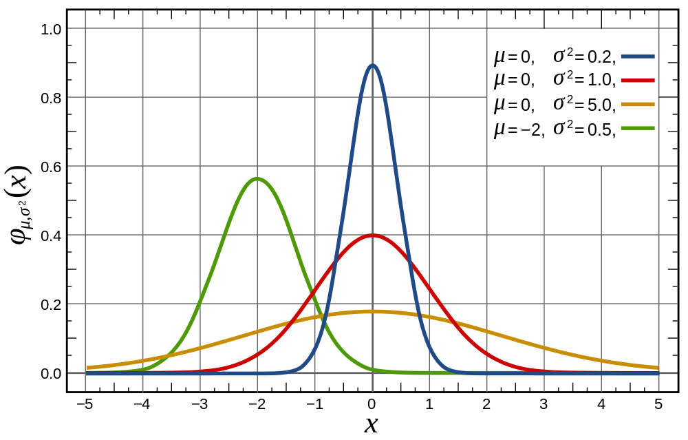
Normal Distribution¶

The normal distribution is often used to approximate the probability distribution of returns.

It is a continuous distribution.

It is symmetric.

It is fully characterized by \(\mu\) (mean) and \(\sigma\) (standard deviation) – i.e. if you only tell me \(\mu\) and \(\sigma\), I can draw every point in the distribution.

Normal Density¶

If \(X\) is normally distributed with mean \(\mu\) and standard deviation \(\sigma\), we write

\[X \sim \mathcal{N}(\mu, \sigma).\]

The probability density function is

\[f(x) = \frac{1}{\sqrt{2\pi} \sigma} \exp\left\{\frac{1}{2\sigma^2}(x - \mu)^2\right\}.\]

Normal Distribution¶

From Wikipedia:

Standard Normal Distribution¶

Suppose \(X \sim \mathcal{N}(\mu, \sigma)\).

Then

\[Z = \frac{X - \mu}{\sigma}\]

is a standard normal random variable: \(Z \sim \mathcal{N}(0,1)\).

That is, \(Z\) has zero mean and unit standard deviation.

We can reverse the process by defining

\[X = \mu + \sigma Z.\]

Standard Normal Distribution - Proof¶

\[\begin{split}E[Z] & = E\left[\frac{X - \mu}{\sigma}\right] \\ & = \frac{1}{\sigma} E[X - \mu] \\ & = \frac{1}{\sigma} (E[X] - \mu) \\ & = \frac{1}{\sigma} (\mu - \mu) \\ & = 0.\end{split}\]

Standard Normal Distribution - Proof¶

\[\begin{split}Var(Z) & = Var\left(\frac{X - \mu}{\sigma}\right) \\ & = Var\left(\frac{X}{\sigma} - \frac{\mu}{\sigma}\right) \\ & = \frac{1}{\sigma^2} Var(X) \\ & = \frac{\sigma^2}{\sigma^2} \\ & = 1.\end{split}\]

Sum of Normals¶

Suppose \(X_i \sim \mathcal{N}(\mu_i, \sigma_i)\) for \(i = 1,\ldots,n\).

Then if we denote \(W = \sum_{i=1}^n X_i\)

\[W \sim \mathcal{N}\left(\sum_{i=1}^n \mu_i, \sqrt{\sum_{i=1}^n \sigma_i^2 + 2\sum_{i=1}^j \sum_{j=1}^n Cov(X_i, X_j)}\right).\]

How does this simplify if \(Cov(X_i, X_j) = 0\) for \(i \neq j\)?

Sample Mean¶

Suppose we don’t know the true probabilities of a distribution, but would like to estimate the mean.

Given a sample of observations, \(\{x_i\}_{i=1}^n\), of random variable \(X\), we can estimate the mean by

\[\hat{\mu} = \frac{1}{n} \sum_{i=1}^n x_i.\]

This is just a simple arithmetic average, or a probability weighted average with equal probabilities: \(\frac{1}{n}\).

But the true mean is a weighted average using actual (most likely, unequal) probabilities. How do we reconcile this?

Sample Mean (Cont.)¶

Given that the sample \(\{x_i\}_{i=1}^n\) was drawn from the distribution of \(X\), the observed values are inherently weighted by the true probabilities (for large samples).

More values in the sample will be drawn from the higher probability regions of the distribution.

So weighting all of the values equally will naturally give more weight to the higher probability outcomes.

Sample Variance¶

Similarly, the sample variance can be defined as

\[\begin{split}\hat{\sigma}^2 & = \frac{1}{n-1} \sum_{i=1}^n (x_i - \hat{\mu})^2.\end{split}\]

Notice that we use \(\frac{1}{n-1}\) instead of \(\frac{1}{n}\) for the sample average.

This is because a simple average using \(\frac{1}{n}\) underestimates the variability of the data because it doesn’t account for extra error involved in estimating \(\hat{\mu}\).

Other Sample Moments¶

Sample standard deviations, covariances and correlations are computed in a similar fashion.

Use the definitions above, replacing expectations with simple averages.